Environmental Engineering Reference
In-Depth Information
P
(
f
)
ρ
(
τ
)
φ
(
t
)
1
0.4
0.8
0.2
0.6
t
0.4
0
00
0.2
−
0.2
0.5
f
50
τ
−
0.4
0.1
0.2
0.3
0.4
10
20
30
40
φ
(
t
)
P
(
f
)
ρ
(
τ
)
3
1
0.08
2
1
0.5
t
0.04
100
200
150
τ
−
1
50
100
−
2
−
0.5
f
−
3
0.04
0.08
φ
(
t
)
P
(
f
)
ρ
(
τ
)
8
1
0.08
4
0.5
t
0.04
100
200
150
τ
50
100
−
4
f
−
0.5
−
8
0.04
0.08
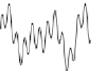
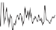
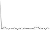
Figure A.1. Examples of power spectrum and autocorrelation function. The rows
refer to the white noise (upper row), deterministic signal (
A.18
) (central row), and
the sum of both (bottom row). From left to right, the columns show a portion of the
signals, the power spectrum, and the autocorrelation function, respectively. The time
is expressed in time units, 4096 samples.
when the signals have infinite energy, the covariance is defined as the mean value of
the covariance function:
T
1
2
T
ρ
(
τ
)
=
lim
T
T
φ
(
t
+
τ
)
φ
(
t
)d
t
.
(A.15)
→∞
−
This expression, divided by
1] is known as the autocorre-
lation function, which is commonly used in signal analysis.
The link between autocovariance and spectrum is given by the Wiener-Khinchin
theorem;
∞
−∞
ρ
φ
2
[in order to have
ρ
(
τ
)
≤
∞
)
e
i
ωτ
d
A
2
(
A
2
(
)
e
−
i
ωτ
d
(
τ
τ
=
ω
)
,
ω
ω
=
ρ
(
τ
)
,
(A.16)
−∞
stating that the energy spectrum is the Fourier transform of the autocovariance, namely
the energy spectrum and autocovariance function form a Fourier pair [i.e.,
ρ
(
τ
)
⇔
A
2
(
ω
)]. Similarly, we can relate the autocorrelation function to the power spectrum
as
∞
−∞
ρ
∞
)
e
i
ωτ
d
)
e
−
i
ωτ
d
(
τ
τ
=
P
(
ω
)
,
P
(
ω
ω
=
ρ
(
τ
)
.
(A.17)
−∞
Figure
A.1
shows some examples of signals along with the corresponding power
spectra and autocorrelation functions. The first row refers to a white noise with zero


Search WWH ::

Custom Search