Environmental Engineering Reference
In-Depth Information
μ
v
,
σ
V
1
0.8
Patterns
0.6
____
No Patterns
V
μ
v
No Patterns
V
V
0
0.4
___
V
0
σ
v
0.2
P
0.2
0.4
0.6
0.8
1
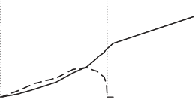
Figure 6.11. Dependence of mean and standard deviation of
v
on the probability
P
of not being in water-stressed conditions (
ζ
=
0
.
4 and same parameters as Fig.
6.10
).
For 0
64 the spatial standard deviation is larger than zero, suggesting the
emergence of spatially heterogeneous vegetation, i.e., pattern formation. The patterns
generated by the model are shown in the insets and include spotted vegetation (inset
on the left,
P
.
2
<
P
<
0
.
=
0
.
375), labyrinthine patterns (central inset,
P
=
0
.
50), and spotted
bare-ground gaps (inset on the right,
P
=
0
.
6). Figure taken from
D'Odorico et al.
(
2006c
).
for mean annual rainfall. Figure
6.11
shows the mean and standard deviation of
as
functions of
P
. For relatively lowvalues of
P
the system is inwater-stressed conditions
for most of the time and vegetation is unable to establish and grow. Thus the system
tends to a uniformly unvegetated state (i.e.,
v
0). For relatively high values
of
P
the system is unstressed for most of the time and vegetation is able to reach
a uniformly vegetated state. In these conditions
v
=
0;
σ
v
=
0 and no patterns emerge. In
intermediate conditions neither one of the two uniform states (vegetated or unvegetated
conditions) can be attained because the repeated switching between the two dynamics
does not allow the system to reach the steady states of the underlying deterministic
dynamics. In this case - depending on the spatial interactions - vegetation may
attain a spatially heterogeneous stable state with a sparse canopy separated by barren
areas. The typical sequence of (noise-induced) patterns along the gradient in mean
annual precipitation (i.e., in the
P
parameter) is shown in Fig.
6.11
(insets). This
sequence ranges from spotted vegetation, to labyrinthine patterns, to spotted gaps.
The widespread occurrence of this type of pattern in dryland ecosystems has been
well documented (e.g.,
Ludwig and Tongway
,
1995
;
Couteron and Lejeune
,
2001
;
Barbier et al.
,
2006
;
Borgogno et al.
,
2009
).
The instability of the state
σ
v
=
v
0
is associated with the emergence of spatial patterns
when the most unstable mode,
k
max
, is different fr
om zero (see
Murray
,
2002
, p. 488).
k
max
can be determined from Eq. (
6.26
),
k
max
=
2log(
χ
4
)
/
(
χ
2
−
1). The condition
of marginal stability [
γ
max
=
γ
(
k
max
)
=
0] becomes
2
χ
4
)
[(1
−
p
)
−
η
P
+
2
η
P
v
0
](
χ
2
χ
−
1
ζ
=
ζ
∗
=
,
(6.27)
πχ
2
(
χ
2
−
1)


Search WWH ::

Custom Search