Environmental Engineering Reference
In-Depth Information
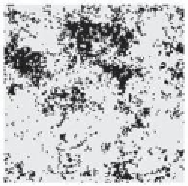
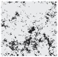
Figure 5.43. Example of pattern resulting from the numerical simulation of model
(
5.87
) under the Ito interpretation. The columns refer to 0, 50, and 100 time units.
The parameters are
a
=
0
.
001,
k
0
=
1,
D
=
25, and
s
gn
=
40.
class of models has a peculiar mathematical structure that reads
∂φ
∂
t
=
)
]
d
V
0
(
φ
)
g
2
(
φ
−
+
L
[
φ
+
g
(
φ
)
ξ
gn
(
r
,
t
)
,
(5.88)
d
φ
where
V
0
is the local deterministic monostable potential with a minimum at
φ
0
,
L
[
φ
]
is the spatial coupling, and
t
) is the usual white (in space and time) Gaussian noise
with zero mean and strength
s
gn
. The key characteristic of these models [Eq. (
5.88
)]
is the function
g
(
ξ
(
r
,
φ
) that modulates, with a different exponent, the three components
of the model: the local deterministic dynamics,
f
(
=−
g
2
(
φ
)
φ
)d
V
0
(
φ
)
/
d
φ
; the noise
ξ
gn
; and the spatial coupling,
g
2
(
component,
g
(
φ
)
φ
)
L
[
φ
]. If functions
V
0
(
φ
)and
g
(
) are suitably chosen, the zero-dimensional component of model (
5.88
) exhibits
noise-induced temporal transitions similar to those of model (
5.73
).
A case investigated in detail (see
Carrillo et al.
,
2003
;
Buceta and Lindenberg
,
2004
) refers to the monostable potential
φ
a
2
φ
2
V
(
φ
)
=
,
(5.89)
with
a
>
0,
1
1
g
(
φ
)
=
(5.90)
+
φ
2
c
[notice that this function is the same as the one in Eq. (
5.73
)], and with Swift-
Hohenberg coupling,
D
(
k
0
+∇
2
)
2
−
φ
. The steady-state pdf of the corresponding
temporal dynamics is
2
)
ν
exp
2
a
φ
p
(
φ
)
=
C
(1
+
c
φ
−
,
(5.91)
2
s
gn
where
C
is the normalization constant and
depends on the interpretation of the noise
term. The pdf (
5.91
) undergoes a noise-induced transition at
s
c
,
t
=
ν
).
The short-term stability analysis of model (
5.88
) with (
5.89
)and(
5.90
)showsthat
the homogeneous solution
a
/
(2
c
ν
φ
=
0 is stable for any noise intensity, whereas the stability
0


Search WWH ::

Custom Search