Noise-induced pattern formation - Noise-induced Phenomena in the Environmental Sciences - page 221

V 0 g φ

2

1

a b

1 0.5

φ φ

2 1 1 2 20 10 10 20

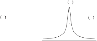
Figure 5.36. (a) Potential corresponding to the local kinetics in model ( 5.73 ) and
(b) behavior of the function g ( φ ). In both cases a = 1 and c = 1.

The local kinetics f ( φ ) =− a φ corresponds to the monostable potential

2

a φ

φ )d φ = V ( φ ) =− f ( , (5.74)

2

φ

showninFig. 5.36 (a). It follows that 0 is the only deterministically

stable ho mogeneous state. Figure 5.36 (b) shows the behavior of the function
g (

φ = φ 0 =

1

φ ) = / (1 + c φ

2 ). It has a maximum at

φ = φ 0 [where g (0) = 1] and decays

symmetrically for increasing values of . We can observe that model ( 5.73 ) does

not exhibit short-term instability. When Eq. ( 5.73 ) is interpreted according to Ito, we
have d

| φ |

φ / d t = f ( φ ) =− a φ , which denotes stability of the basic state φ = 0

(recall that a 0). Also, when the Stratonovich interpretation is adopted, following

the methods in Box 5.4, we obtain
d

>

φ
d t

c φ

=− a φ − s gn

2 ) 2 ;

(5.75)

+ φ

(1 c

because the spurious drift term is also negative, it is unable to destabilize the basic
state.
The purely temporal component of model ( 5.73 ), namely

1
1

d d t =−

a φ +

2 ξ gn ( t )

, (5.76)

+ c φ

exhibits a noise-induced bistability. In fact, the steady-state pdf is

2 ) ν exp

φ

2 (2

+ φ

2 )

a c

p ( φ ) = C (1 + c φ − , (5.77)

4 s gn

where C is the normalization constant and 1, depending on the use of

the Stratonovich or Ito interpretation, respectively. The modes

ν = 1 / 2or ν =

φ m correspond to the

zeros of

2 ν cs gn φ m

− a φ m + = 0 . (5.78)

m ) 2

2

(1 + c φ