Noise-induced pattern formation - Noise-induced Phenomena in the Environmental Sciences - page 217

pdf pdf

p d f

0.8 0.8

60

30

0.0 φ

2 φ 2 φ

0.02

2 2

S S S

1

6000 6000

0.5 3000 3000

1 k 1 k

3 k

0.5 0.5

1 2

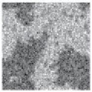
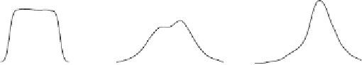
Figure 5.33. Numerical simulations of the diffusive VPT model. The columns refer
to 0, 50, and 200 time units ( s gn =

5, and the other conditions are as in
Fig. 5.10 ). The gray-tone scale spans the interval [

2, D =

− 2 , 2].

For simplicity, in this section we consider processes driven by symmetrical DMN, i.e.,
processes with k 1 = k 2 = k and =− = ; the corresponding noise intensity 1 2

2 . Other forms of colored noise could of course be used to represent the
temporal correlation of the random forcing, but the results would be analogous to
those found with DMN.
The four models considered are
∂φ
∂

is s dn =

D ( k 0 +∇

2 ) 2

t =

a φ − φ + ξ dn , (5.69)

∂φ
∂

2

t =

a φ + D ∇ φ + ξ dn , (5.70)

∂φ
∂

3

D ( k 0 +∇

2 ) 2

t =

a φ − φ + φξ dn − φ, (5.71)

∂φ
∂

3 2

t =−

a φ − φ + φξ + D ∇ φ, (5.72) dn

which correspond to prototype models ( 5.16 ), ( 5.29 ), ( 5.34 ), and ( 5.58 ), respectively,
analyzed in previous sections.