Noise-induced pattern formation - Noise-induced Phenomena in the Environmental Sciences - page 213

pdf pdf

p d f

60

1.4

30

0.0 φ

2 φ 2 φ

0.02

2 2

S S S

1.5

8000 8000

1

4000 4000

0.5

1 k 1 k

3 k

0.5 0.5

1 2

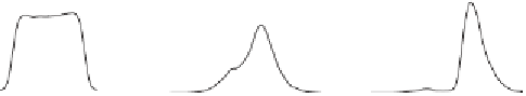
Figure 5.30. Example of numerical simulations of the prototype model ( 5.58 ). The
columns refer to 0, 10, and 40 time units ( s gn = 5, and the other

conditions are as in Fig. 5.10 ). The gray-tone scale spans the interval [

2 , a =− 1 , D =

− 2 , 2].

instability tends to disappear, the spatial patterns follow the same fate and tend to
fade out. In the long term the only legacy of the effect of the spatial coupling on the
dynamics can be found in the phase transition (i.e., m

=

0), though it is associated

with a homogeneous field.
It is also worth noticing two other features of the patterns shown in Fig. 5.30 . First,
even though they are multiscale patterns, their main wave numbers are always close
to zero. Thus the dominant wavelengths observable in the simulated fields are always
of the same order of magnitude as the domain size. This is consistent with dispersion
relation ( 5.60 ), which exhibits positive growth rates close to the maximum at k 0.

Therefore these noise-induced multiscale patterns fall into the category of spatial
structures (see Subsection 5.1.1 ) with no clear dominant wavelengths. These stochastic
models can provide a suitable representation of some real transient patterns found in
the environmental sciences. The second interesting aspect concerns the boundaries of
the geometrical features existing in patterns induced by multiplicative noise. Similar
to the case discussed in Subsection 5.4.1 , the coherence regions are much sharper and
less fringed than those observed in the case of additive noise (compare Figs. 5.16 and
5.30 ). Also in this case, the difference is due to the multiplicative nature of the noise,
which means that the g (

=

φ ) ξ gn term is spatially correlated.