Environmental Engineering Reference
In-Depth Information
γ
1
s
gn
1.5
k
0.5
1
1.5
s
gn
1
s
gn
0.5
1
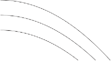
Figure 5.29. Dispersion relation for prototype model (
5.58
) for three values of the
noise intensity
s
gn
(
a
=−
1,
D
=
1).
pattern-forming spatial interactions. In other words, the spatial coupling would not
be able to induce patterns in the deterministic counterpart of the system. Thus we
consider models with the same temporal component,
f
(
ξ
m
, as those studied
in Section
5.4
. This allows us to compare the results with those presented in Section
5.4
and to stress the role of the type of spatial coupling. In particular, we choose
the diffusive differential operator,
φ
)
+
g
(
φ
)
2
, as the exemplifying case of non-
pattern-forming coupling. Similar to the case investigated in Subsection
5.4.1
,the
prototype model is then
L
[
φ
]
=
D
∇
φ
∂φ
∂
3
2
t
=
a
φ
−
φ
+
φξ
+
D
∇
φ,
(5.58)
gn
where
a
is a parameter and
ξ
gn
is zero-mean white Gaussian noise, with intensity
s
gn
. Equation (
5.58
) is interpreted in the Stratonovich sense. The homogeneous deter-
ministic stable state of Eq. (
5.58
)is
φ
0
=
0, and short-term instability occurs when
s
gn
>
a
(see Subsection
5.4.1
).
We first study the linear stability of the basic state
s
c
=−
φ
0
in the dynamics of the
ensemble average. Because of the linearity of the spatial coupling, such dynamics are
described by
∂
φ
∂
t
3
2
=
a
φ
−
φ
+
s
gn
φ
+
D
∇
φ
.
(5.59)
The stability analysis of (
5.59
) leads to the dispersion relation
Dk
2
γ
(
k
)
=
a
+
s
gn
−
.
(5.60)
Figure
5.29
shows some examples of dispersion relation (
5.60
) calculated for dif-
ferent noise intensities
s
gn
. Three properties are evident. First, the value
s
gn
a
of the noise intensity marks the condition of marginal stability: No u
nstable wave
numbers occur when
s
gn
=−
a
, whereas the wave numbers lower than
(
s
gn
<
−
+
a
)
/
D


Search WWH ::

Custom Search