Environmental Engineering Reference
In-Depth Information
p
d
f
p
d
f
p
d
f
0.5
0.5
60
30
0.0
φ
2.5
φ
2.5
φ
0.02
2.5
2.5
S
S
S
1
800
800
0.5
3
k
3
k
3
k
1
2
1
2
1
2
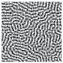
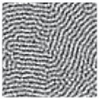
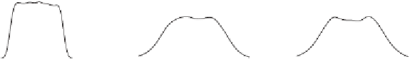
Figure 5.27. Patterns obtained from numerical simulation of the VPT model with
spatial coupling a la Swift-Hohenberg. The columns correspond to
t
=
0
,
10, and
100 time units. The rows show the field, the pdf of the variable
φ
, and the azimuth-
averaged spectrum, respectively. The parameters are
k
0
=
1,
s
gn
=
2
.
5,
D
=
15, and
=
1 (the other conditions are as in Fig.
5.10
). The gray-tone scale spans the interval
[
−
2
,
2].
an ordered (i.e., patterned) state requires both spatial coupling (i.e.,
D
needs to exceed
a noise-dependent critical value) and intermediate noise intensities.
It is also interesting to notice that the classical form of the mean-field technique
(Box 5.4) indicates that model (
5.49
) is unable to exhibit phase transitions in the sense
defined in Subsection
5.1.3
.Infact,usingEq.(
5.28
) with
f
(
φ
i
)givenby
Eq. (
5.49
), we obtain the fact that the order parameter
m
remains equal to zero for
any value of
s
gn
and
D
.
Figure
5.27
shows some numerical simulations of Eq. (
5.49
). Both a visual inspec-
tion of the field and an analysis of its power spectrum averaged over the azimuthal
angle clearly show the occurrence of a distinct periodic pattern. The wavelength
2
φ
i
)and
g
(
28 pixels corresponds to the one identified by linear-stability analysis
and remains stable in time. The pattern is stochastically steady (i.e., it maintains its
average characteristics), although the fronts of the coherence regions continuously
π/
k
max
=
6
.


Search WWH ::

Custom Search