Environmental Engineering Reference
In-Depth Information
γ
1
s
gn
0.9
k
0.5
1
1.5
2
s
gn
0.5
1
s
gn
0.1
2
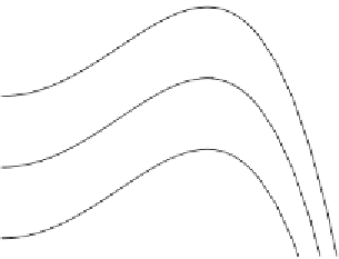
Figure 5.25. Dispersion relation of the VPT model with spatial coupling `alaSwift-
Hohenberg for three values of noise standard deviation (
D
=
1,
k
0
=
1).
Figure
5.24
(b) shows an example of the steady-state pdf corresponding to model
(
5.52
):
2
2
s
gn
1
+
φ
e
−
p
(
φ
)
=
√
2
s
gn
]
,
(5.53)
1
π
(1
+
φ
2
)erfc[
where erfc[
0for
any noise intensity, which confirms that perturbations of the deterministic stable state
φ
·
] is the complementary error function. The pdf has the mode at
φ
=
s
c
.
To investigate the ability of dynamics (
5.49
) to generate periodic patterns, we focus
on the deterministic differential equation describing the spatiotemporal dynamics
of
0
tend to disappear in spite of their initial amplification when
s
gn
>
φ
:
∂
φ
∂
t
=−
φ
1
2
φ
1
−
2
2
D
(
k
0
+∇
2
)
2
+
φ
+
2
s
gn
+
φ
φ
.
(5.54)
The dispersion relation obtained by use of the techniques described in Box 5.1 is
D
(
k
0
−
k
2
)
2
γ
(
k
)
=−
1
+
2
s
gn
−
.
(5.55)
If we focus on positive wave numbers, the maximum is localized at
k
max
=
k
0
,where
γ
(
k
=
k
max
)
=
2
s
gn
−
1 (see Fig.
5.25
). It follows that (i) unstable wave numbers
occur only if
s
gn
>
5 and (ii) the selected pattern is periodic with a wavelength
approximatively equal to
0
.
k
max
. The first condition is the same as the one
obtained from the short-term analysis and confirms that pattern formation needs
short-term instability, namely patterns are absent if noise intensity is subthreshold
(i.e.,
s
gn
<
λ
=
2
π/
5).
The generalized mean-field technique is useful for understanding the role of the
intensity both of noise
s
gn
and of the spatial coupling
D
(
Parrondo et al.
,
1996
). If this
technique is applied to VPT model (
5.49
) and the most unstable modes are considered
s
c
=
0
.


Search WWH ::

Custom Search