Environmental Engineering Reference
In-Depth Information
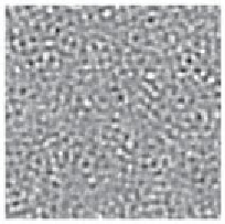
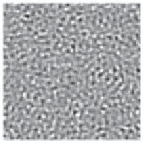
Figure 5.23. Numerical simulation of model (
5.46
). The parameters are
a
=−
1,
5. The three panels correspond to
t
equal to 0, 10, and
100 time units. The gray-tone scale is in the interval [
D
=
10,
k
0
=
1, and
s
gn
=
0
.
−
0
.
3
,
0
.
3].
φ
φ
term
f
(
) close to
0
. For example, consider the model
∂φ
∂
3
1
/
3
D
(
k
0
+∇
2
)
2
t
=
a
φ
−
φ
+
φ
×
ξ
gn
−
φ.
(5.46)
In this case the short-term analysis yields
d
φ
d
t
s
gn
3
≈
a
φ
−
φ
+
=
f
eff
(
φ
)
.
(5.47)
/
3
φ
1
3
It follows that
d
f
eff
d
φ
=+∞
,
lim
φ
→
φ
(5.48)
0
and the short-term behavior is then unstable for any noise intensity (i.e., even when
s
c
=
0), indicating that the noise component always overwhelms
f
(
φ
)when
φ
is close
to zero. Notice that the balance between
f
(
φ
)and
g
(
φ
)
ξ
is reversed when
φ
moves
away from
0. This fact hampers the divergence of the system. The numerical
simulation shown in Fig.
5.23
confirms that model (
5.46
) generates stable patterns
with the same dominant wavelength as those shown in Fig.
5.20
.
φ
=
0
5.4.3 Case with g
(
φ
0
)
=
0
: The van den Broeck-Parrondo-Toral model
In this subsection, we study a more complex model with respect to the one investigated
in Subsection
5.4.1
. It is shown that more complicated forms of the functions
f
(
φ
)
and
g
(
) do not qualitatively change the picture drawn in the previous subsections,
provided that the interplay between short-term instability and spatial coupling remains
the same. To this end, we can consider the stochastic model
φ
∂φ
∂
2
)
2
2
)
D
(
k
0
+∇
2
)
2
t
=−
φ
(1
+
φ
+
(1
+
φ
×
ξ
−
.
(5.49)
gn


Search WWH ::

Custom Search