Noise-induced pattern formation - Noise-induced Phenomena in the Environmental Sciences - page 197

0

s m s c ,D 0

s m s c ,D 0

s m s c ,D 0

t

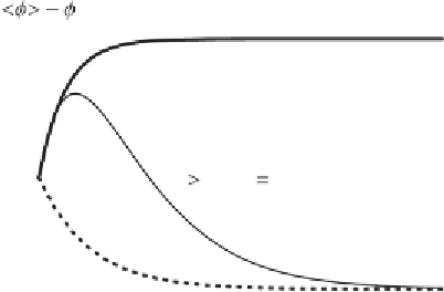
Figure 5.17. Scheme of the possible evolutions of small initial displacement depend-
ing on the noise intensity and the strength of the spatial coupling.

that noise-induced instability is transient, in the sense that the state 0 is recovered in

the long term. This behavior is shown by the thin continuous curve in Fig. 5.17 :Noise
initially induces a growth (i.e., an instability) of

φ

φ

,butfor t →∞ the difference

| φ − φ 0 | tends to zero. This behavior (i) explains why this mechanism is called

short-term instability and (ii) suggests that the steady-state pdf of φ is expected to be

unimodal, with the mode at φ 0 ,evenwhen s m exceeds the threshold s c .

We now consider spatiotemporal dynamics (i.e., D = 0). Differently from the

subcritical case, when s m > s c , the spatial coupling introduces qualitative changes with

respect to the zero-dimensional case. In fact, for suitable values of the strength D of the
coupling, the spatial term in Eq. ( 5.31 ) takes advantage of the noise-induced short-term
instability that also exists in the spatiotemporal dynamics (in fact, ∂ φ /∂ t d φ / d t

for t from decaying to zero. As a

consequence, the spatial coupling locks the system in a new ordered state, with

→ 0) and prevents the displacement | φ − φ 0 |

φ

different from φ 0 and variable in space. In this case the temporal trajectory of φ does

not exhibit a convergence to , as shown by the thick curve in Fig. 5.17 .

Thus the spatial coupling is responsible for maintaining the dynamics away from the
state

φ

0 for t

→∞

0 . Before investigating the behavior of some prototype models, we describe in
Box 5.5 an analytical tool used to detect the possible presence of short-term instability
in stochastic dynamical systems.
Once the short-term instability has been detected, the ability of spatiotemporal
stochastic dynamics ( B5.5-1 ) to give rise to periodic patterns is typically investigated
by the prognostic tools described in Boxes 5.1, 5.2, and 5.3.

φ

5.4.1 Prototype model
To illustrate howpattern formation can be induced bymultiplicative noise, we consider
the prototype model:

∂φ
∂

3

D ( k 0 +∇

2 ) 2

t =

a φ − φ + φξ gn − φ, (5.34)