Environmental Engineering Reference
In-Depth Information
S
st
i
p
b
a
60
1.2
40
0.8
20
0.4
2.5
k
D
0.5
1
1.5
2
5
10
15
20
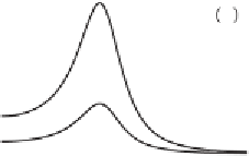
Figure 5.14. (a) Shape of the structure function at steady state for model (
5.16
)
with
L
[
φ
] given by expression (
5.6
); the upper curve corresponds to
s
gn
=
3, the
lower one to
s
gn
=
1(
k
0
=
1
,
a
=−
1
,
D
=
3). (b) Dependence of the peak intensity
on strength of spatial coupling
D
for
k
0
=
2; the solid, dotted, and dashed curves
correspond to
a
=−
0
.
01
,
−
0
.
1, and
−
1, respectively.
(homogeneous) basic state
0. Notice that
i
p
depends on
a
,
D
,and
k
0
but not
on the noise intensity
s
gn
; therefore, although noise is necessary for the emergence of
patterns, it does not affect pattern intensity.
We observe that, in this case, pattern occurrence cannot be detected through the
analysis of the dynamics of the ensemble mean
φ
0
=
. In fact, by taking the ensem-
ble average of Eq. (
5.16
), in the case of a zero-mean additive noise we obtain
(see Box 5.1)
φ
∂
φ
∂
t
2
k
0
)
2
=
a
φ
−
D
(
∇
+
φ
,
(5.22)
which is an equation formally identical to the deterministic part of original model
(
5.16
), in which the effect of the noise is completely hidden. Therefore the conditions
controlling the stability and instability of the zero-mean (i.e.,
0) homogeneous
state are the same as those controlling the stability of the homogeneous state
φ
=
0in
(
5.16
). Thus, using the ensemble mean to detect noise-induced changes, the stochastic
dynamical system would not seem to be able to generate stable patterns when
a
φ
=
<
0.
The generalized mean-field technique is also unable to detect the constructive
(i.e., pattern-forming) role of additive noise. In fact, the application of this technique
(see Box 5.3) leads to
φ
d
i
d
t
=
a
φ
i
−
D
ω
(
k
)
φ
i
−
D
eff
(
φ
i
−
φ
i
)
+
ξ
gn
,
i
,
(5.23)
where
k
0
−
k
y
)]
2
2
ω
(
k
)
=
2
[2
−
cos(
k
x
)
−
cos(
,
(5.24)
D
4
(
k
)
k
0
2
4
D
eff
=
2
−
+
4
−
ω
.
(5.25)


Search WWH ::

Custom Search