Noise-induced pattern formation - Noise-induced Phenomena in the Environmental Sciences - page 187

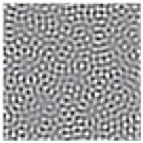
Figure 5.10. Dynamics described by model ( 5.17 ) when a is negative ( a =− 0 . 1,

D = 10, k 0 = 1). The three panels correspond to t equal to 0, 5, and 35 time units, the

field has 128 128 pixels, and periodic boundary conditions are set. The gray-tone

scale spans the interval [10 − 3

×

10 3 ]. The initial condition is , φ ( r , t = 0) = ξ u , where

ξ u is a noise uniformly distributed in the interval [10 − 2 10 2 ].

,

tend to vanish as the system tends to the homogeneous stable state φ = 0. Notice that

the transient pattern exhibits the periodicity of about 2 π/ k 0 pixels imposed by the

spatial coupling (see Appendix B).
Conversely, when a is positive no steady states exist and the dynamics of diverge.

However, even in this case the spatial terms in ( 5.17 ) are able to induce patterns
that become more and more pronounced (i.e., with stronger spatial gradients) as the
dynamics diverge (see Fig. 5.11 ). To stabilize the dynamics to a steady state, it is
necessary to introduce a nonlinear term that hampers the dynamics in diverging.
A relatively simple nonlinear term is

φ

3 ; in this case the dynamics turn into the
celebrated Ginzburg-Landau model, with local dynamics expressed as f (

− φ

φ ) = a φ −

3 ,

φ

∂φ
∂

3 2

k 0 ) 2

t =

a φ − φ − D ( ∇ + φ. (5.18)

− √ a , √ a ] - the diverging effect of the lin- For small values of φ - in the interval [

ear term a φ prevails (with a > 0), and as φ increases the stabilizing effect of the

Figure 5.11. Example of the dynamics described by deterministic model ( 5.17 ) when
a is positive ( a

=+ . =

10, k 0 = 1). The three panels correspond to t equal to

0, 30, and 60 time units, and the gray-tone scale spans the interval [

0 1, D

− . , .

0 1 0 1]. The

other conditions are as in Fig. 5.10 .