Environmental Engineering Reference
In-Depth Information
φ
φ
1
1
a
b
15
x
15
x
15
15
0.1
0.1
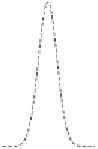
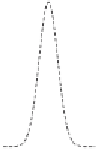
Figure 5.6. Example of the effect of (a) the Laplacian term and (b) the fourth-
derivative term. Panel (a) refers to equation
2
x
2
∂φ/∂
t
=
∂
φ/∂
and panel (b) to
4
x
4
. In both panels the initial condition (a bell-shaped
the model
∂φ/∂
t
=−
∂
φ/∂
x
2
distribution,
2]), is shown with the dashed curve, and the solid curves
refer to the solution after 5 time units.
φ
=
exp[
−
/
x
2
φ
have a bell-shaped distribution,
φ
[
x
,
t
=
0]
=
exp[
−
/
2]. The field is subjected to
∇
2
φ
∂φ/∂
=
∂
2
φ/∂
x
2
, and the distribution of
φ
a diffusive term
, i.e.,
t
is investigated
=
at
t
5 time units. As expected, the Laplacian operator has the effect of producing a
redistribution of
φ
along the
x
axis, with a smoothing of the peak and an increase of
spatial coherence.
A mathematical structure that is useful in the description of pattern-forming
couplings is
2
4
L
φ
=−
∇
φ
−∇
φ,
[
]
a
0
(5.4)
4
is the so-called biharmonic term, equal to
where
a
0
is a parameter and
∇
φ
=
∂
4
φ
∂
4
φ
y
2
+
∂
4
φ
4
∇
+
2
y
4
.
(5.5)
∂
x
4
∂
x
2
∂
∂
4
If we reconsider the same example as before, but with
, the result in
Fig.
5.6
(b) is obtained. It is evident that the spatial coupling in this case produces
coherent structures with a clear periodicity, i.e., periodic patterns (see Appendix B).
Note that all the spatial-coupling operators considered so far have the property
that they do not affect a spatially homogeneous field. In fact,
∂φ/∂
t
=−∇
φ
L
[
φ
]
=
0 if the field is
homogeneous. In contrast, the Swift-Hohenberg operator,
2
k
0
)
2
L
[
φ
]
=−
(
∇
+
φ
(5.6)
(where
k
0
is a parameter), does not have this property, but can be decomposed into
a pattern-forming term of the form of Eq. (
5.4
) (with
a
0
2
k
0
) plus a drift term
=
k
0
φ
.
Other examples of mathematical operators that can be used to express the spatial
coupling is provided by the integral operator
f
(
φ
)
=−
(
r
)
r
)d
r
,
L
[
φ
(
r
)]
=
φ
ω
(
r
−
(5.7)


Search WWH ::

Custom Search