Noise-induced phenomena in environmental systems - Noise-induced Phenomena in the Environmental Sciences - page 160

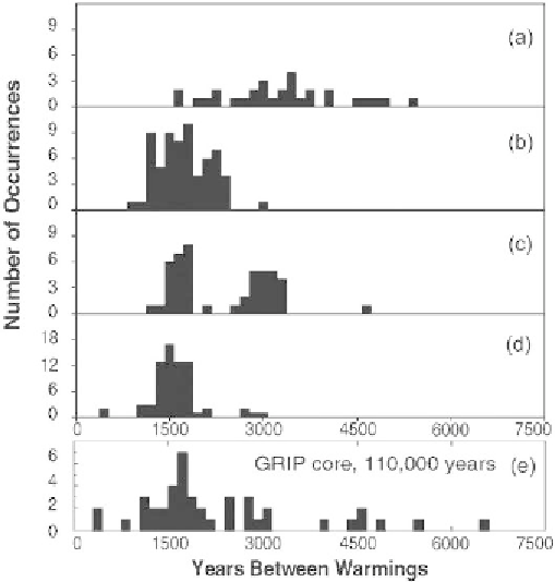
Figure 4.29. Probability distribution of the interspike times between consecutive
DO events based on simulations with (a) relatively weak noise (noise intensity
s gn = 10 − 3 )

and no periodic forcing; (c) both periodic and “weak” stochastic forcing (

10 − 4 ) and no periodic forcing; (b) stronger noise ( s gn = 6 . 125 × 1 . 25 ×

σ =

10 − 3 );
(e) interspike time distribution obtained from the analysis of Greenland ice-core
project (GRIP) data from Alley et al. ( 2001 ). Figure taken from Ganopolski and
Rahmstorf ( 2002 ).

10 − 4 ); (d) both periodic and “strong” stochastic forcing ( 6 . 125 × σ = 1 . 25 ×

the absence of an external periodic forcing, the noise term may induce temporary
transitions to the unstable circulation mode. Interestingly, when the noise levels (i.e.,
variance) are sufficiently high, the distribution of waiting times between DO events
is clustered in the 1000-2500-yr range (Fig. 4.29 ). Thus noise is able to enhance and
unveil an intrinsic waiting time time between DO occurrences. Moreover, this waiting
time is close to the observed 1500-yr periodicity [Fig. 4.29 (e)]. Thus this analysis
would suggest that the periodic DO events are an example of coherence resonance
( Timmermann et al. , 2003 ). However, the analysis of ice-core data shows the exis-
tence of smaller modes at 3000 and 4500 yr in the waiting-time distribution of DO
events. These modes could emerge as an effect of stochastic resonance. Ganopolski
and Rahmstorf ( 2002 ) forced their global-climate model both with (additive) noise
and with periodic fluctuations in freshwater inputs. They found that the three modes
appear for adequate noise levels, consistent with the analysis of ice-core records
[Figs. 4.29 (c)-(e)]. Although, by itself, this weak periodic forcing is not able to