Environmental Engineering Reference
In-Depth Information
A
m
a
1
0.8
0.6
0.4
______
Stable
Unstable
s
c
0.2
s
gn
1
2
3
4
5
6
7
p
A
2.5
b
2
1.5
1
______
s
gn
0.5
s
c
0.5
s
gn
8.0
s
c
A
0.2
0.4
0.6
0.8
1
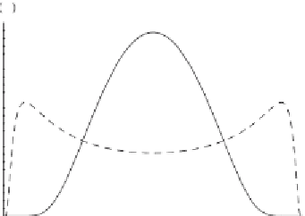
Figure 4.22. Stochastic genetic model: (a) stable and unstable states of the system as
a function of the noise intensity (
s
gn
), (b) pdf of
φ
with
a
0
=
0,
β
=
0
.
5 (in this case
s
c
=
2).
becomes unstable and two new stable states emerge. The steady-state probability
distribution of
A
can be determined from Eq. (
2.83
):
s
gn
1
−
β
A
1
1
s
gn
(
a
0
1
s
gn
(
a
0
Ce
−
+
+
2
β
−
1)
−
1
A
)
−
+
2
β
−
1)
−
1
p
(
A
)
=
A
(1
−
,
(4.34)
1
−
A
where
C
is the normalization constant. Figure
4.22
(b) shows some examples of
probability distributions of
A
, which become bimodal when
s
gn
exceeds
s
c
, indicating
the occurrence of noise-induced bistability.
We note that in a number of systems the harvest rate is a nonlinear function of
A
.
For example, the consumption by predators is likely to reach saturation for high values
of
A
as the predator needs are met (
Ludwig et al.
,
1978
). To account for this saturation
effect the harvest rate can be expressed as
kA
b
A
b
), as suggested for the case of
insect outbreak dynamics (
Ludwig et al.
,
1978
). Interesting noise-induced transitions
may also emerge in these systems when in Eq. (
4.28
) the coefficient
k
(instead of
a
)
is treated as a (Gaussian) random variable to account for the effect of rapidly varying
(random) environmental conditions. These dynamics were investigated in detail by
Horsthemke and Lefever
(
1984
) in the context of predator-prey systems. We refer
/
(1
+


Search WWH ::

Custom Search