Environmental Engineering Reference
In-Depth Information
p H
a
f H
c
6
5
0.0025
4
_____
0.0045
H
P
...........
0.0065
3
_____
f H a H b
1
H
2
1
1
H
1
H
0.2
0.4
0.6
0.8
0.2
0.4
0.6
0.8
p
H
b
p H
d
7
6
λ
a
_____
0.1;
b
0.01
6
5
____
0.30
5
4
______
0.20
4
λ
a
3
............
0.05
3
0.5;
b
0.05
2
2
1
1
1
H
1
H
0.2
0.4
0.6
0.8
0.2
0.4
0.6
0.8
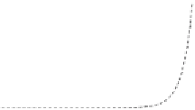
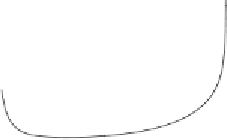
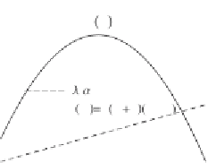
Figure 4.15. (a), (b) Probability distribution of soil thickness
H
calculatedwith (
4.17
)
for different values of
λ
and
α
:(a)
α
=
0
.
05,
a
=
0
.
0012, and
b
=
0
.
05; (b)
λ
=
0
.
001,
a
=
0
.
0012, and
b
=
0
.
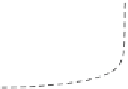
05; (c) stable state of the deterministic process with
state-dependent erosion rate
H
: The stable state is obtained as intersection (point
P
in the figure) between the soil-production function
f
(
H
) and the deterministic
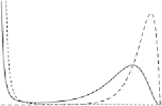
erosion rate. (d) Probability distribution of soil thickness calculated with (
4.18
).
λα
We can investigate the deterministic counterpart of these dynamics by replacing
the stochastic rates of erosion with their average value
. Thus these determinis-
tic dynamics have only one stable state between 0 and 1, which is determined as
the solution of the equation
f
(
H
)
λα
−
λα
=
0. In the case of stochastic dynamics, a
second preferential state emerges at
H
=
0. This state is induced by the bound of
the multiplicative Poisson noise (
h
≤
H
), which translates into the existence of a
probability “atom” at
h
H
in the distribution
p
(
h
)of
h
(see Fig.
4.14
). Because
this bound corresponds to a state dependency in the effect of the random forcing
on the process
H
(
t
), the dynamics of
H
are driven by multiplicative noise. More-
over, although the stable state of the deterministic dynamics is always smaller than
1, Fig.
4.15
(b) shows examples of bistable stochastic dynamics with a stable state at
H
=
1. Thus the stable states of the stochastic and deterministic dynamics are not the
same.
We now consider a similar process in which landslides are modeled as random
(Poisson) occurrences, with each landslide removing the whole soil column. In fact,
observational evidence indicates that the failure surface usually coincides with the
regolith-bedrock interface (e.g.,
O'Loughlin and Pearce
,
1976
;
Sidle and Swanston
,
1982
;
Trustrum and De Rose
,
1988
). In this case the distribution of the Poissonian
jumps
h
is
p
(
h
)
=
=
δ
(
h
−
H
). Alternatively, the process could be expressed by (
4.9
)


Search WWH ::

Custom Search