Environmental Engineering Reference
In-Depth Information
2
4
a
1
P
1
1
I
V
III
a
2
4
P
1
1
a
1
1.5
p B
p B
p B
B
B
B
a
2
1
II
0.5
p B
p B
B
IV
B
0.2
0.4
0.6
0.8
1
P
1
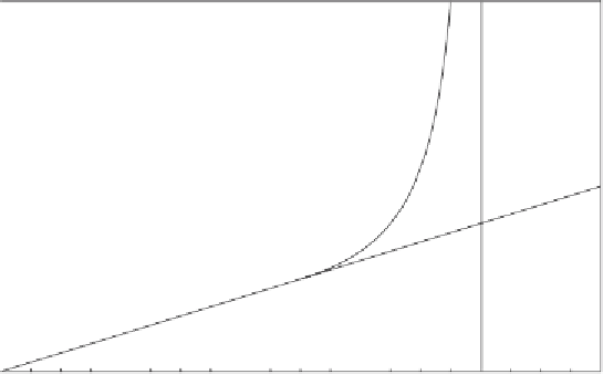
Figure 4.1. Shapes of the probability distributions of biomass
B
as functions of the
parameters
P
1
and
a
2
of the state-independent dichotomous process (calculated for
a
1
=
2). A variety of dynamics can be obtained, includings L-shaped distributions
with preferential state at
B
0
.
=
0 (case I), J-shaped distributions with preferential state
at
B
1 (case II), bistable dynamics with bimodal (U-shaped) distribution (case III),
dynamics with only one stable state located between the extremes of the domain of
B
(case IV), bimodal distributions with a preferential state at
B
=
=
0 and the other for
B
<
1 (case V).
a
1
(Fig.
4.1
, case II). When both conditions are met,
p
(
B
)is
U-shaped with two spikes of probability at
B
B
=
1) for
P
1
>
1
−
=
=
1(Fig.
4.1
, case III).
When none of these conditions is met, the probability distribution of
B
has only one
mode within the interval [0, 1] and no spikes of probability at
B
=
0and
B
0orat
B
=
1
(Fig.
4.1
, case IV). It can be shown that when
p
(
B
) has a singularity at
B
=
0(but
not at
B
a
1
)],
p
(
B
) has both a mode and an
antimode in [0, 1], as in Fig.
4.1
(case V). This mode and the spikes of
p
(
B
) in cases
I, II, and III are preferential (i.e., more probable) states of the system, and we interpret
them as statistically stable states of the dynamics.
Because the probability distribution of
B
exhibits different shapes depending on
the values of the parameters
a
1
,
a
2
,and
P
1
(Fig.
4.1
), the preferential states of
B
vary
across the parameter space. For relatively low (high) rates of decay
a
2
and high (low)
probability
P
1
of occurrence of unstressed conditions, the dynamics have a preferential
state (i.e., spike of probability) in
B
=
1) and
a
2
<
(4
a
1
P
1
−
1)
/
[4(
P
1
−
1
−
0). In intermediate conditions the
system may exhibit either one (case IV) or two (case III and V) statistically stable
states. This bistability [i.e., bimodality in
p
(
B
)] emerges as a noise-induced effect
(see Chapter 3) and is an example of the ability of noise to induce new states, which
do not exist in the underlying deterministic system (
Horsthemke and Lefever
,
1984
).
=
1(
B
=


Search WWH ::

Custom Search