Information Technology Reference
In-Depth Information
0.85
m=9, n=20
0.8
0.75
0.7
0.65
0.6
0.55
0.5
1
2
3
4
5
6
7
8
9
Auction
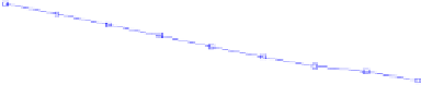
Fig. 3.
The winner's expected profit for the normal distribution
198
m=9,n=20
m=9, n=19
m=9, n=18
197.5
197
196.5
1
2
3
4
5
6
7
8
9
Auction
Fig. 4.
Revenue for a varying competition
and the difference between the first and second highest order statistics is [5]:
E
(
s
n
)=
n
∞
−∞
E
(
f
n
)
[
F
(
x
)]
n−
1
[1
−
−
F
(
x
)]
dx
(15)
We substitute these values for
E
(
s
n
) and
E
(
f
n
)
E
(
s
n
) to find the expected revenue
and the winner's expected profit for each individual auction in a series.
The variation in the revenue for different auctions is shown in Figure 1. As shown
in the figure, the expected revenue decreases from one auction to the next. A bidder's
cumulative ex-ante expected profit from auctions
j
to
m
(i.e.,
α
j
) is shown in Figure 2.
This profit decreases from one auction to the next. The winner's expected profit also
drifts downward as shown in Figure 3.
−
The effect of competition.
In order to study the effect of competition, we fix the number
of objects (
m
) and vary the number of bidders (
n
) for the example scenario described
above. Figure 4 is a plot of the expected revenue for different
n
. As seen in the figure,
for all the three values of
n
(i.e.,
n
=20,
n
=19,and
n
=18) the seller's revenue
declines from one auction to the next. Figure 5 is a plot of the winner's expected profit