Information Technology Reference
In-Depth Information
Posterior Probability
P
(
v
|
l
w
,
F
(
x
)
,
L
)
Actual Number Of Bidders (
n
)
30
0.12
d.
a. Prior
b. Posterior after 2 auctions
c. Posterior after 4 auctions
d. Posterior after 20 auctions
0.1
20
0.08
10
1
5
10
15
20
Repeated Auctions
c.
0.06
Bid Levels & Observed Closing Prices (
L
,
l
w
)
4
0.04
b.
3
0.02
a.
2
0
1
5
10
15
20
0
20
40
60
80
100
Repeated Auctions
Mean Number Of Bidders
(v)
(a)
(b)
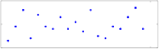
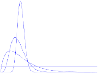
Fig. 4.
Plots showing (a) the actual number of bidders that participated in the auction (unknown
to the auctioneer) and the actual bid levels and closing prices observed by the auctioneer and (b)
the prior and posterior belief distributions of the auctioneer after 2, 4 and 20 repeated auctions
ability distribution. However, for our purposes, we calculate it as a discrete probability
distribution over a suitable range. In this example, we calculate
P
(
ν
|
l
w
,
F
(
x
)
,
L
) for
integer values of
ν
from
ν
to
ν
. Thus, this normalising factor is given by:
t
i
=1
P
l
i
w
|
ν
,
F
(
x
)
,
l
i
P
(ν)
ν
ν=ν
Z
=
(11)
Finally,
P
(
ν
) represents the auctioneers' prior belief; an initial assumption as to which
values of
are most likely to occur, before any observations have been made. If no such
intuition is available (as in our simulations here), the prior can simply be initialised as
a uniform distribution, and it will have no effect on the estimates generated.
Thus the procedure adopted by the auctioneer is as follows: it first uses its prior belief
(i.e. an initial guess) to calculate the bid levels for the first auction. Having observed the
closing price of this auction, the expression in equation 10 is used to calculate the prob-
ability distribution that describes its updated belief in the parameter
ν
ν
. This probability
distribution is then used to choose the value of
for the calculation of the optimal bid
levels to be implemented in the next auction. There are two ways in which this choice
can be made, either: (i) the most likely value of
ν
ν
can be used (i.e. the value of
ν
where
the probability distribution has a maximum), or (ii) a value of
may be sampled from
this probability distribution. The first option is identical to a statistical maximum like-
lihood estimator. However the second option ensures more rapid convergence in cases
where the auctions that occur early in the learning process represent extreme events (i.e.
when many of the bidders have extremely high or low valuations or the auction happens
to have many more or many less bidders than is typical).
Simulation results for this procedure are shown in figure 4. Here, we consider the
same uniform valuation distribution as discussed in section 5 (i.e.
x
= 0and
x
= 4).
Therealvalueof
ν
in this case is 20, whilst the auctioneer's prior belief is that it lies
somewhere between 0 and 100 (i.e.
P
(
ν
ν
) is a uniform distribution over this range). In