Information Technology Reference
In-Depth Information
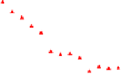
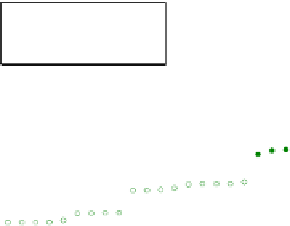
Average Daily Offer Price ($/cycle)
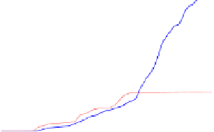
Cumulative Order Quantity (cycles)
x 10
4
500
15
SouthamptonSCM
FreeAgent
Mr.UMBC
SouthamptonSCM
FreeAgent
Mr.UMBC
12
400
9
300
6
200
3
100
0
0
40
80
120
160
200
0
40
80
120
160
200
Simulation Day
Simulation Day
(a)
(b)
x 10
7
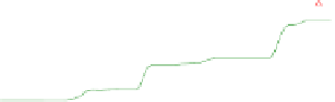
Cumulative Order Revenue ($)
3
SouthamptonSCM
FreeAgent
Mr.UMBC
2.4
1.8
1.2
0.6
0
0
40
80
120
160
200
Simulation Day
(c)
Fig. 2.
Comparison of offer prices, quantity and revenue in game 1136
pricing model is particularly successful. The prices offered by SouthamptonSCM are
just low enough that the offers of the competing agents are undercut, but high enough
that the resulting orders generate as much revenue as possible.
After analysing more semi-final games, we found that the prices SouthamptonSCM
offers follow the same broad trend compared with the other two. And, in particular, the
trend is when the customer demand is high, the prices are high, and vice versa. This
can be seen from Figure 2 (a), where the demand for the first half of the game is high,
and the demand decreases gradually till Day 160 and increases again. Accordingly, the
prices are high before Day 110 and then start to decrease gradually. At the end of the
game, although the demand is increasing, the agents do not increase their prices because
they want to offload their stock. Moreover, in most of the games we considered, the
prices SouthamptonSCM offered just undercut the other two. This is also reflected by
the quantity of orders our agent won which was again usually the highest.
4.3
Controlled Experiments
To evaluate the performance of our agent in a more systematic fashion than is possible
in the competition, we decided to run a series of controlled experiments. As mentioned