Analysis 02: OWF Effect on the Ocean - On the Effect of Offshore Wind Farms on the Atmosphere and Ocean Dynamics - page 122

a b

c

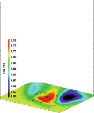
Fig. 5.47 (a) HAMSOM SST in three-dimensional illustration. Square of solid lines mark OWF
in the middle of the area, which is surrounded by dotted square , indicating sections by 6-km
difference to OWF. Additionally, a square of dashed-dotted lines highlights closest SST, com-
pared to CTD measurements. Illustration (b) and (c) picture HAMSOM SST along squares of (a).
Illustration (b) shows HAMSOM SST along the section in 6-km distance to OWF. Illustration (c)
shows HAMSOM SST along the section with a distance of y ¼ 12 km from the OWF to the

Δ

northern section, y ¼ 3 km to the southern section, and x ¼ 15 km to western section, and

Δ Δ

Δ 12 km to eastern section. Little black squares mark the OWF position in (b) and (c). Results

are based on three days of operating wind turbine simulation

x ¼

that these corners are outside of the main downwelling cell, where the model shows
weak positive vertical velocities.
With using the it appears to be too small to detect the

upwelling cell being expected south/southeast of the wind farm, as model
results show.
Overall, the agreement between simulation and measurements is impressive,
considering the theoretical model setup and computational restriction and the
observed temperature profiles linked to downwelling within and around alpha
ventus .

6 km-distance square,

' '

References

Backhaus J (1985) A three-dimensional model for the simulation of shelf sea dynamics. Ocean
Dyn 38:165-187. doi: 10.1007/BF02328975
Brostr¨m G (2008) On the influence of large wind farms on the upper ocean circulation. J Marine
Syst 74:585-591