Analysis 02: OWF Effect on the Ocean - On the Effect of Offshore Wind Farms on the Atmosphere and Ocean Dynamics - page 83

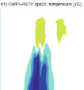
Fig. 5.21 Hovm¨ ller diagrams of OWF effect (OWFr-REFr) of hydrographic depending on three
different cases of OWF operation opc01 (a1-a3), opc02 (b1-b3), and opc03 (c1-c3) along the S-
N cross section. Illustration (a1)-(c1) show results of SST, (a2)-(c2) of salinity at the surface, and
(a3)-(c3) of density at the surface. Horizontal black lines clarify mode of OWF operation. Here,
the solid lines show the start of OWF operation mode, while the dashed horizontal lines stand for
switching off/ignoring the OWF. The OWF district is around y 0 km and counts 12 wind

turbines. Maximal changes occur parallel to extreme changes of surface elevation

¼

In a time difference of 14 h, a weaker extrema of exist, weakened over 7 more

hours, followed by an increase again to a little weaker extrema than before. Extrema
are placed close to the OWF, but depending on the first

ζ

duration, the horizontal
is differently affected in the three operation cases. The pulsing of

on

' '

is connected
with the vertical cells. Changes in surface elevation and velocity field are concen-
trated at the OWF region; only surface elevation affects more horizontal area
by time.

ζ

Fig. 5.20 (continued) operation mode, while dashed horizontal lines stand for switching
off/ignoring the OWF. The OWF district is around y ¼ 0 km and counts 12 wind turbines. While
horizontal velocity component u acts with wind forcing, maximum changes of the residual
dynamical variables occur time shifted. After 1.8 days without OWF signal, the OWF signal on
the ocean still exists, albeit weaker