Selection of Visual Descriptors for the Purpose of Multi-camera Object Re-identification - Feature Selection for Data and Pattern Recognition - page 265

DCT

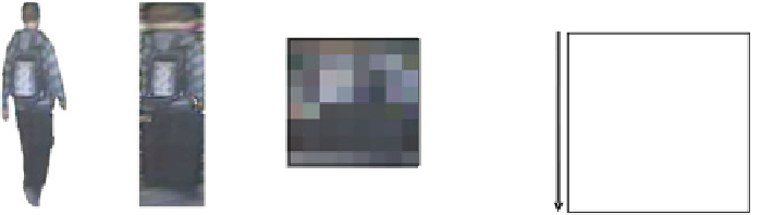
Fig. 12.5 Consecutive stages of Colour Layout Descriptor calculation. From left described object,
its stretched representation, image regions mean calculation, and the DCT coefficient scanning
result

As the CLD is defined for images of defined rectangular dimensions and the
object shape can vary, the visual object representation is stretched in each row to
defined dimensions during the preprocessing stage. Afterwards, the analysed image
is divided into equal blocks (8

8). Next, a representative value for each image region
is calculated as the mean channel intensity within a block. As a result, image thumb-
nail is acquired, which is further transformed using DCT (discrete cosine transform).
To form the feature vector, coefficients scanning, along with their normalization is
performed. This type of coefficient reading method is utilized to group low fre-
quency components together. The final feature vector acquired this way consists of
192 elements, in which 64 DCT coefficients for each colour channel are included. In
MPEG-7 standard it is stated that for CLD descriptor, YCbCr representation should
be used ( CLD descriptor). For the purpose of experiments, besides YCbCr, addi-
tionally Transformed Colour, defined by Eq. 12.3 , is utilized as well ( CLDTrans
descriptor).

×

12.4.5 Co-occurrence Matrices Statistical Parameters

This image descriptor contains statistical parameters of co-occurrence matrices of
an object image ( CMSP descriptor). A co-occurrence matrix, also referred to as a
co-occurrence distribution, is defined over an image to be the distribution of co-
occurring values at a given offset (

Δ x , Δ y )[ 13 , 25 ]. It is commonly used as a

texture description.
A set of symmetrical, normalized, co-occurrence matrices P is calculated for each
channel of the object image in HSV colour space. Each set contains four matrices P
calculated for four different directions of offsets: 0 ⓦ —offset (0,1), 45 ⓦ —(1,1), 90 ⓦ —
(1,0) and 135 ⓦ —(1,

− 1). Image values are quantized into 16 × 16 equally-spaced

levels, therefore each co-occurrence matrix contains 16 16 elements. Example

co-occurrence matrices P for two different object images are visualised in Figs. 12.6
and 12.7 .

×