Biomedical Engineering Reference
In-Depth Information
120
40
100
30
80
60
20
40
10
20
0.015
0.02
0.025
0.03
0.015
0.02
0.025
0.03
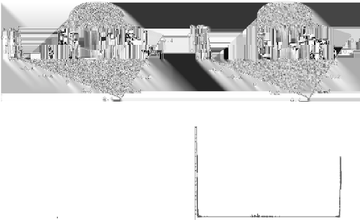
Figure 11.17: The graph of the segmentation function and its histograms in
time steps 100 and 200 for the same experiment as presented in Fig. 11.16.
The histograms give a practical advise to shorten the segmentation process in
case of noisy images. For a noisy image, the formation of completely piecewise
flat subjective surface takes longer time. However, the gaps in histogram of the
segmentation function are developed soon. It allows to take any level inside these
gaps and to visualize the corresponding level line to get desirable segmentation
result (color slide).
As can be seen in Fig. 11.18, in our method the centers of pixels are con-
nected by a new rectangular mesh and every new rectangle is splitted into
four triangles. The centers of pixels will be called degree of freedom (DF)
nodes. By this procedure we also get further nodes (at crossing of red lines
in Fig. 11.18) which, however, will not represent degrees of freedom. We will
call them non-degree of freedom (NDF) nodes. Let a function
u
be given by
discrete values in the pixel centers, i.e. in DF nodes. Then in additional NDF
nodes we take the average value of the neighboring DF nodal values. By such
defined values in NDF nodes, a piecewise linear approximation
u
h
of
u
on the
triangulation can be built. Let us note that we restrict further considerations
in this chapter only to this type of grids. For triangulation
T
h
, given by the pre-
vious construction, we construct a co-volume (dual) mesh. We modify a basic