Biomedical Engineering Reference
In-Depth Information
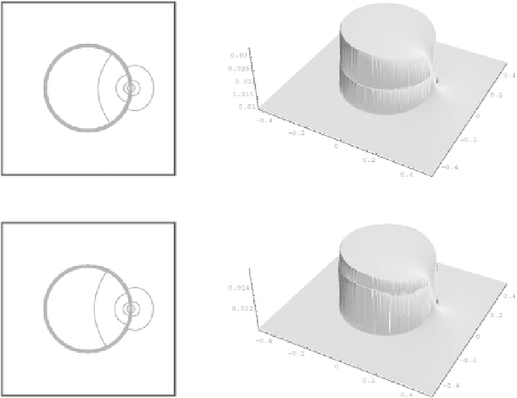
Figure 11.13: Experiment on testing image plotted in Fig. 11.12 (left). The
results of evolution of the segmentation function (in the left its isolines, in the
right its graphs) after 10 (top row) and 100 (bottom row) time steps. In this case,
ε
=
1, the shape is stable, but moving downwards in a “self-similar” form, so it
is not utilizable as the segmentation result.
very good segmentation results as presented in Fig. 11.14. Of course, smaller
ε
is needed to close larger gaps (see Fig. 11.15).
If there is a noisy image as in Fig. 11.12 (right), the motion of level lines to
shock is more irregular, but finally the segmentation function is smoothed as well
(see Figs. 11.16 and 11.17). If the regularization parameter
ε
is small, then piece-
wise flat profile of the segmentation function will move very slowly downwards,
so it is easy to stop the evolution and get the result of segmentation process.
In the presented experiments, we have seen that the solution of Eq. (11.2)
is well suited to finding and completing edges in (noisy) images. Its advection-
diffusion mechanism leads to promising results. In the next section we give an
efficient and robust computational method for its solution.