Biomedical Engineering Reference
In-Depth Information
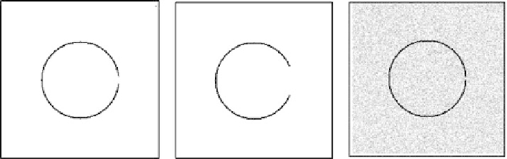
Figure 11.12: Three testing images. Circle with a smaller (left) and a big (mid-
dle) gap, and noisy circle with a gap.
the smoothing is applied only outside the edges. On the edges the advection
dominates, since the mean curvature term is multiplied by a small value of
g
0
.
In Fig. 11.11 ( bottom) we may see formation of a piecewise flat profile of the
segmentation function, which can be again very simply used for extraction of
“batman,” although, due to Dirichlet boundary data and
ε
=
1, this profile moves
slowly downwards in subsequent evolution. In this (academic) example, the only
goal was to smooth (flatten) the segmentation function inside and outside the
edge, so the choice
ε
=
1 was really satisfactory. In the case
ε
=
1, Eq. (11.2) can
be interpreted as a time relaxation for the minimization of the weighted area
functional
g
0
1
+|∇
u
|
A
g
0
2
dx
,
=
or as the mean curvature motion of a graph in Riemann space with metric
g
0
δ
ij
[48].
In the next three testing images plotted in Fig. 11.12 we illustrate the role
of the regularization parameter
ε
. The same choice,
ε
=
1, as in the previous
image with complete edge, is clearly not appropriate for image object with a
gap (Fig. 11.12 (left)), as seen in Fig. 11.13. We see that minimal-surface-like
diffusion closes the gap with a smoothly varying “waterfall” like shape. Although
this shape is in a sense stable (it moves downwards in a “self-similar form”), it
is not appropriate for segmentation purposes. However, decreasing
ε
, i.e., if we
stay closer to the curvature-driven level set flow (11.8), or in other words, if
we stretch the Riemannian metric
g
0
δ
ij
in the vertical
z
direction [49], we get