Biomedical Engineering Reference
In-Depth Information
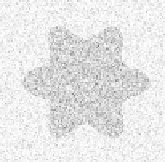
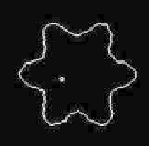
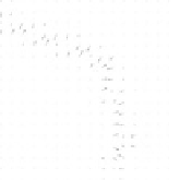
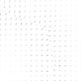
Figure 10.12: Region force diffusion—top row: A synthetic image with additive
Gaussian noise, region segmentation map, region boundary map
R
, and gradient
of the region map
R
(and a small selected area)—bottom row: diffused region
vector field, and close-up views in the small selected area of the vectors in the
gradient of region map and the diffused region vector field respectively.
where
x
and
y
are the spatial sample intervals,
p
max
is the maximum of
p
(
·
),
and
t
is time step, the interval between time
t
n
and time
t
n
+
1
when iteratively
solving (10.12).
From (10.11) and (10.12) we note that within a homogeneous region, based on
the criteria of region segmentation,
p
(
·
) equals 1 while
q
(
·
) equals 0. Thus (10.12)
is only left with the first term (as the second term vanishes). This effectively
smooths the vector field. However, at the region boundaries,
p
(
·
)
→
0 and
q
(
·
)
→
1. The smoothing term imposes less and the region vectors are close to the
gradient of the region map
R
. Thus the diffused region vector field provides
the evolving snake with an attracting force in a sufficiently large range near
the region boundaries, and also allows the snake to evolve solely under other
gradient forces.
Figure 10.12 illustrates an example of region force diffusion, including close-
up views of pre- and post-diffusion vector field.
10.4.3 Region-Aided Snake Formulation
Next, we can derive the region-aided geometric snake formulation. The standard
geometric snake is given by (10.8). In the traditional sense, the snake forces fall