Biomedical Engineering Reference
In-Depth Information
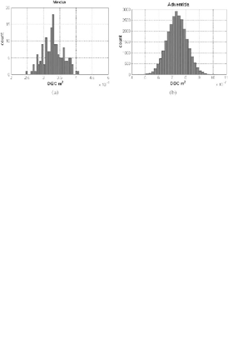
Figure 1.28:
DBC distributions of simulated arterial structures: media (a) and
adventitia (b).
Table 1.4. The typical cell nuclear size was obtained by Perelman
et al.
[22].
In Fig. 1.29 we can observe the dependency of axial resolution and the ultra-
sound frequency. To illustrate this, four IVUS simulated images are shown.
Low
frequency
ranging from 10 to 20 MHz corresponds to an axial resolution from
154 to 77
µ
m, and
intermediate frequency
from 20 to 30 MHz gives axial res-
olution from 77 to 51
µ
m. In these cases, it is possible to visualize accumu-
lations around 100 RBCs.
High frequency
from 30 to 50 MHz leads to 51-31
µ
m of axial resolution. Moreover, it is now possible to visualize accumula-
tions of tens of RBCs. The IVUS appearance improves when the frequency in-
creases, allowing different structures and tissue transition interfaces to be better
detected.
Table 1.4:
Typical IVUS simulation magnitudes
Parameter
Magnitude
Ultrasound speed
1540 m/sec
Maximal penetration depth
2E
−
2m
Transducer angular velocity
1800 rpm
Transducer emission radius
3E
−
4m
Attenuation coefficient
α
0.8 dB/MHz cm
Ultrasound frequency
10-50 MHz
Beam scan number
160-400
Video noise
8 gray level
Instrumental noise
12.8 gray level
Beta parameter
38
5ad
β
=
.