Biomedical Engineering Reference
In-Depth Information
d
r
=
c
/
f
able to be measured when the frequency
f
and the ultrasound speed
c
are known. Taken typical values for
c
=
1540 m
/
sec and frequency of 40 MHz,
V
o
≈
2
.
39
×
10
−
4
mm
3
, thus
N
o
≈
370 “voxels.”
1.5 Simulation of IVUS Image
1.5.1 Generation of the Simulated Arterial Structure
Considering the goal of simulating different arterial structures, we can classify
them into three groups: tissue structures, nontissue structures, and artifacts.
The spatial distribution of the scatterer number with a given DBC,
σ
(
R
,,
Z
)
at point (
R
,
,
Z
), has the following contributions:
σ
(
R
,,
Z
)
=
A
(
R
)
+
B
(
R
,,
Z
)
+
C
(
R
)
(1.11)
where
A
(
R
)
,
B
(
R
,θ,
Z
), and
C
(
R
) are the contributions of tissue structures,
nontissue structures, and artifacts respectively.
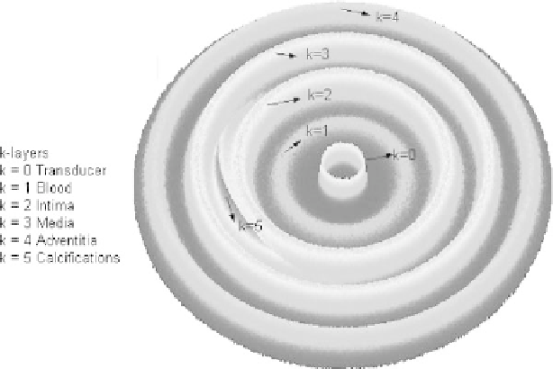
1.
Tissue scatterers
. These are determined by the contribution of the normal
artery structures, corresponding to
lumen, intima, media, and adventi-
tia
. Figure 1.20 shows a
k
-layers spatial distribution of the scatterers for a
simulated arterial image. These scatterers are simulated as radial Gaussian
Figure 1.20:
A plane of
k
-layers simulated artery. The scatterer numbers are
represented by the height coordinate in the figure.