Biomedical Engineering Reference
In-Depth Information
1
1
1
0.5
0.5
0.5
0
0
0
−
0.5
−
0.5
−
0.5
−
1
−
1
−
1
−
1
−
0.5
0
0.5
1
−
1
−
0.5
0
0.5
1
−
1
−
0.5
0
0.5
1
(a)
(b)
(c)
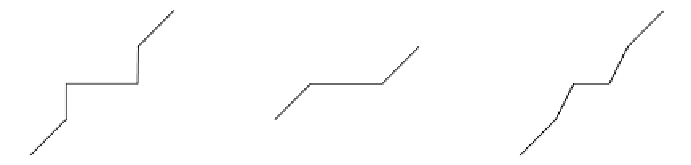
Figure 6.10: Example of thresholding functions, assuming that the input data
was normalized to the range of [
−
1, 1]. (a) Hard thresholding, (b) soft thresh-
olding, and (c) affine thresholding. The threshold level was set to
T
=
0
.
5.
therefore reflects the “strength” of signal variation. For second-derivative-based
wavelets, the magnitude is related to the local contrast around a signal varia-
tion. In both cases, large wavelet coefficient magnitude occurs around strong
edges. To enhance weak edges or subtle objects buried in the background, an
enhancement function should be designed such that wavelet coefficients within
certain magnitude range are amplified.
General guidelines for designing a nonlinear enhancement function
E
(
x
)
are [35]:
1. An area of low contrast should be enhanced more than an area of high con-
trast. This is equivalent to saying that smaller values of wavelet coefficients
should be assigned larger gains.
2. A sharp edge should not be blurred.
In addition, an enhancement function may be further subjected to the following
constraints [36]:
1. Monotonically increasing: Monoticity ensures the preservation of the rel-
ative strength of signal variations and avoids changing location of local
extrema or creating new extrema.
2. Antisymmetry: (
E
(
−
x
)
=−
E
(
x
)): This property preserves the phase po-
larity for “edge crispening.”
A simple piecewise linear function [37] that satisfies these conditions is plotted
in Fig. 6.11(a):
⎧
⎨
x
−
(
K
−
1)
T
,
if
x
<
−
T
E
(
x
)
=
Kx
,
if
|
x
|≤
T
.
(6.39)
⎩
x
+
(
K
−
1)
T
,
if
x
>
T