Shape From Shading Models - Biomedical Image Analysis - page 268

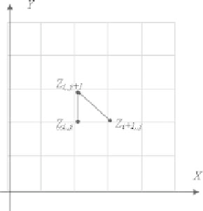
Figure 5.1:

The grid mesh for the discretization in Example 3.

methods used to solve these matrix equations, for example, the Jacobi method,
can be found in the standard numerical analysis textbooks [24].

For a nonlinear shape from shading model (5.5), we have to linearize the
reflectance map by using Taylor expansion to get a linear equation and then apply
the FDM in a similar way as in the above example. To linearize the equation, we
only need to replace the nonlinear part in Eq. (5.2) by its linear approximation.
We first rewrite the equation to separate the linear and nonlinear parts:
I ( x , y ) 1 + p 0 + q 0 1 + p 2 + q 2 = ρ (1 + p 0 p + q 0 q ) . (5.30)

Denoting the nonlinear part by

1 + p 2

F ( p , q ): = + q 2

,

the Taylor expansion of F ( p , q )at( p , q )is

F ( p , q ) = F ( p , q ) + ( p − p ) F p ( p , q ) + ( q − q ) F q ( p , q )
+ O ( | ( p − p ) 2 + ( q − q ) 2

| )

(5.31)

1 + p 2

p
1 + p 0 + q 0 + ( q − q )

q
1 + p 0 + q 0 , + q 2 ≈ + ( p − p )

where the error term O ( | ( p − p ) 2

+ ( q − q ) 2 | ) depends on the value of ( p , q )

and the smoothness of the solution function Z . If we assume that Z ∈ C 2 ( ) ,
then this error term can be ignored locally. Now we substitute (5.30) into (5.31)
to have the linearized irradiance equation:

P ( x , y ) p + Q ( x , y ) q = I ( x , y ) , (5.32)