Recent Advances in the Level Set Method - Biomedical Image Analysis - page 235

( x*,y* ) ( x*, y* )

1 2 1 2

(a) (b)

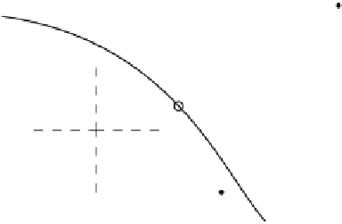
Figure 4.20: Choice of stencil for (a) points not crossed by the interface and (b)
points where the interface crosses the stencil. Dashed lines indicate the points
used in the stencil.

These equations are solved for γ i − 1 , γ i , γ i + 1 , and C i , thus determining the nu-
merical approximation corresponding to the point x i using Eq. 4.62. A similar
process is followed for the approximation centered at x i + 1 . This results in a
specialized discretization at these two points and standard central difference
approximations everywhere else.
For higher dimensional problems, a similar approach is taken. At grid points
not crossed by the interface, the standard central difference stencil is used (see
Fig. 4.20(a)) to approximate Eq. 4.58. At grid points where the interface crosses
through the stencil, an additional grid point is chosen across the interface from
the center of the stencil (see Fig. 4.20(b)).
When building the specialized discretization for the stencil at grid points
as in Fig. 4.20(b), a point ( x ∗ , y ∗ ) is chosen for the point around which the
approximation will be computed, and around which all Taylor expansions will be
taken. Usually, the point ( x ∗ , y ∗ ) is the point on the interface closest to the center
of the stencil (in this example, point 2). Once ( x ∗ , y ∗ ) is chosen, a coordinate
transformation is taken so that the interface normal maps onto the x -axis. Once
this coordinate transformation is completed, the computation of the stencil is
similar to the one-dimensional case described above.
As noted earlier, the advantage of this method is that it is truly second-order
accurate, even in the neighborhood of the interface. However, the stencil that
is produced is irregular, and it sometimes can be difficult to solve the resulting
linear system. Also, the choice of the points ( x ∗ , y ∗ ) is somewhat arbitrary, and