Civil Engineering Reference
In-Depth Information
ρ
V
v
C
p
∂
T
∂
t
=−
A
s
[
h
(
T
−
T
∞
)
]
−
2
kA
c
∂
2
T
T
4
−
T
4
∞
−
A
s
ε
r
σ
SB
+ (
1
− ξ)
VI
∂
x
j
(5.24)
where
ρ
is the density of the material,
V
v
is the volume of the part,
C
p
is the spe-
cific heat of the material,
T
is the temperature,
t
is time,
A
s
is the exposed sur-
face of the part,
h
is the convection heat transfer coefficient,
T
∞
is the surrounding
temperature,
k
is thermal conductivity of the die material,
A
c
is the cross-sectional
area,
x
j
are coordinates,
ε
r
is radiative emissivity for the part,
σ
SB
is the Stefan-
Boltzmann constant,
V
is the electric voltage, and
I
is the intensity of the current,
given by the product of the current density and cross-sectional area.
The goal of this subsection is to determine the significance of each of the three
heat transfer modes. To determine this, Eq. (
5.24
) was modified in the model to
represent the following heat transfer mode combinations and then compared to
experimental results:
• All heat transfer modes except radiation (Eq.
5.25
)
• All heat transfer modes except radiation and convection (Eq.
5.26
)
• All heat transfer modes except conduction (Eq.
5.27
)
ρ
V
v
C
p
∂
T
∂
t
=−
A
s
[
h
(
T
−
T
∞
)
]
−
2
kA
c
∂
2
T
+ (
1
− ξ)
VI
(5.25)
∂
x
j
ρ
V
v
C
p
∂
T
∂
t
=−
2
kA
c
∂
2
T
+
(
1
−
ξ)
VI
(5.26)
∂
x
j
ρ
V
v
C
p
∂
T
T
4
−
T
4
∞
∂
t
=−
A
s
[
h
(
T
−
T
∞
)
]
−
A
s
ε
r
σ
SB
+ (
1
− ξ)
VI
(5.27)
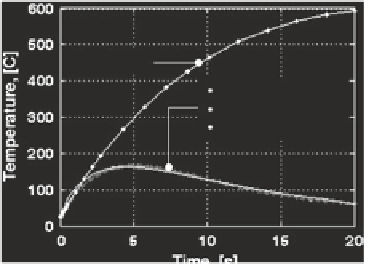
The resulting thermal profiles for all of the combinations are displayed in Fig.
5.18
.
From the figure, the experimental temperature profile and the profiles neglecting
Fig. 5.18
EAF heat transfer
modes analysis [
11
]. Thermal
profiles for stationary
electrical tests were
calculated without particular
heat transfer modes to
identify the most significant
mode (conduction)
w/out cond.
Experiments
All H/T modes
w/out rad. and conv