Civil Engineering Reference
In-Depth Information
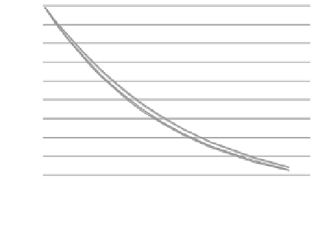
Fig. 5.3
Specimen resistance
change with respect to
strain and temperature 0
[
1
]. Although the overall
normalized resistances
change with the strain
(because of the decreasing
specimen height), there is
no notable difference in
resistance change in relation
to the specimen temperature
(different current densities)
100%
90%
80%
27.7 A /mm2
35.8 A /mm2
54.6 A /mm2
60.8 A /mm2
70%
60%
50%
40%
30%
20%
10%
0%
0
0.2
0.4
0.6
0.8
1
1.2
True Strain
1
+
2
µ
r
0
3
h
inst
J
∗
=
F u
+ ξ ·
P
e
=σ
π
r
inst
(5.16)
where the effective stress will be given by Eq. (
5.11
). Thus, Eq. (
5.17
) can be writ-
ten as follows:
1
+
2
µ
r
0
3
h
inst
F u
+ ξ
VI
=
C
ε
n
ε
m
π
r
inst
(5.17)
where
V
and
I
are the voltage and current intensity. The current is given by Eq. (
5.18
):
Amps
mm
2
I
=
π
r
inst
C
d
[
=
]
mm
2
·
(5.18)
with
C
d
being the current density (i.e., current/cross-sectional area) and
π
r
inst
being the cross-sectional area of the workpiece. Equations (
5.10
), (
5.17
), and
(
5.18
) constitute the analytical model for an electrically assisted compression test.
5.1.8 Overall Solution Schematic
A MATLAB program was implemented to numerically solve the equations derived
for the model using an incremental approach. By imposing the material and ini-
tial dimensions of the part, the model is used to determine the effective strain
and stress for different current density values. The solution schematic is given in
Fig.
5.4
. A mechanical power step,
P
m
, is preset such that
P
m
increases incre-
mentally throughout the test. In particular, the overall mechanical power pro-
file is divided into a given number of steps, at which mechanical forces will be
determined. More steps will produce higher modeling accuracy; however, it will
increase modeling time. At step
i
,
Eq. (
5.10
) is solved to determine the temperature
rise and then used to find the corresponding strength coefficient,
C
. The new value