Wire Ropes Under Bending and Tensile Stresses - Wire Ropes: Tension, Endurance, Reliability - page 266

99.9

99.5
99

[%]

95
90
80
70
60
50
40
30
20
10
5

N' = 44% ʽ = 1,06
N' = 55% ʽ = 1,26
N' = 70% ʽ = 1,38

N' = 88% = 1,28

birth distribution
Poisson distribution

ʽ

Seale 8x19 − IWRC − sZ
lubricated viscous min. oil
reverse bending l = 300 d
d = 12 mm, D/d =25
steel hardened, r = 0.53 d
tensile stress ˃ z = 484 N/mm 2

1

0.5

0.1

0 10 20

number of wire breaks B 6

30 40

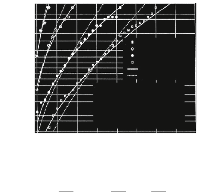
Fig. 3.75 Comparison of wire breaks distribution with Poisson and birth distribution, Ren ( 1996 )

v 1 Þ ¼C ð B L Þ C ð B L

B L B L

v 1 Þ:

b ð B L ;

v 1 Þ= C ð B L þ

The probability that the number of wire breaks is smaller or equal to B L is

p ð B L Þ ¼ X

B L

w ð B L Þ; ð 3 : 79a Þ

0

and the probable number of wire breaks B L,max on the reference length L is given
again by ( 3.82 ), now with p(B L ) from ( 3.79a ).
The observed numbers of wire breaks, which can be explained through the
Poisson-distribution or the birth-distribution, are regarded as normal since they are
the result of the natural process of the occurrence of wire breaks, Ren ( 1996 ).
Those breaks which are not able to be explained, even by the birth distribution, are
described with the term ''dangerous break concentrations''. These weak points can
be discovered at an early stage. Figure 3.76 shows the percentage of the wire break
distributions in a series of bending fatigue tests that Ren ( 1996 ) was able to explain
by either the Poisson or, at least, by the birth-distribution.