Wire Ropes Under Bending and Tensile Stresses - Wire Ropes: Tension, Endurance, Reliability - page 265

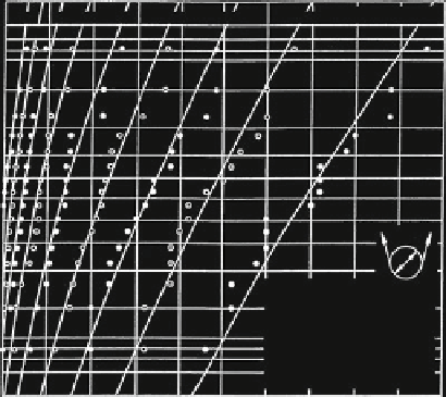
Fig. 3.74 Number of wire
breaks distribution and
Poisson distribution

99
98
95

x10 3

50 80 100 125 160 200 250 N= 320

63

90

80
70

60

50
40
30
20

S=30kN

D

I = 8 x 2 x 22.5 d
Warrington 8 x 19
SFC − sZ, bright
d = 16 mm, D/d = 25
steel, r = 0.53 d
lubricated

10
5
2
1 0

5 10 15 20

number of wire breaks B 22.5

25 30 35 40 45 50

According to ( 3.82a ), the probable maximum number of wire breaks is
B L,max = 11. The probable maximum number of wire breaks can be calculated
with the help of the Excel-program, ''POISSON 2.XLS''.
Figure 3.74 shows the distribution of the wire breaks observed in a bending
fatigue test and the calculated Poisson distribution with ( 3.79 ) drawn as smooth
curve. This figure shows just how closely the observed number of wire breaks
corresponds to the Poisson distribution close to the end of the rope life.
Very often the Poisson distribution is valid only for the smaller relative number
of bending cycles. An example for this is to be seen in Fig. 3.75 where the
observed numbers of wire breaks already deviate from the Poisson distribution for
the relative number of bending cycles N 0 = 55 %. However these observed
numbers of wire breaks can be explained as a birth-distribution introduced by Ren
( 1996 ).
For the birth-distribution, the wire breaks continue to occur by chance but
prefer those sections already weakened by w ir e breaks. For the birthdistribution,
Ren ( 1996 ) defined the variance factorm ¼ V = B L where the variance is greater than
the mean number of wire breaks V [ B L . Remember, m = 1 for the Poisson-
distribution.
The probability w(B L ) of the birth-distribution that the number of wire breaks
B L = 0, 1, 2, 3, etc. exists on the reference length L is according to Ren ( 1996 )

B L

1 v 1

v

B L
v v 1

w ð B L Þ ¼ ð 3 : 77a Þ

B L

b ð B L ;

v 1 Þ B L

with the Beta-function expressed by the better known Gamma-function C