Geoscience Reference
In-Depth Information
ϕ
xy
are frequency-dependent and have been estimated from the
spectra of the two input signals. Characteristically, geodetic and atmospheric exci-
tation show a remarkably high coherence (
c
xy
functions
c
xy
and
=
0
.
94
−
0
.
97) and small phase
25
◦
)at
T
lag values (
365d, suggesting that the atmosphere is a major
driving agent for the excitation of prograde and retrograde annual wobbles. Indeed,
the amplitude of the observed prograde wobble excitation is in excellent agreement
with that of the equatorial AAM, while there is more inconsistency in the retro-
grade band, see Gross et al. (
2003
). Significant values of
c
xy
are present at other
spectral bands that feature high signal-to-noise ratios, such as semi- and terannual
frequencies. The polar motion variations allocated to these bands can be explained
to about 60% by atmospheric pressure and wind fluctuations, as noted for instance
in Eubanks (
1993
). Further intraseasonal wobbling motion is also partially driven
by atmospheric processes, with surface pressure variations over Eurasia and North
America of particular importance, see Nastula and Salstein (
1999
). At such time
scales from several weeks to months, Fig.
11
reveals only minor phase lag values
but limited coherences of about 0.5 at positive frequencies and 0.6 at negative fre-
quencies. This implies that non-atmospheric processes such as oceanic excitation
should be considered, too, see Sect.
3.4
for a short look at the angular momentum
contributions of Earth's other subsystems. The invalidity of the inverted barometer
approximation at very short periods is reflected in the substantial drop of coherence
at about 10d.
A brief illustration of the integration approach (Eq.
80
) is given in Fig.
12
.It
employs the same geodetic and geophysical data as the previous example. The
numerical integration required for convolution can be performed via Simpson's rule,
and both the observed polar motion series as well as its corresponding atmospheric
ϕ
xy
=±
≈
0.5
0
Observation
Excitation
−0.5
0.6
0.4
0.2
0
−
0.2
1980
1985
1990
1995
2000
2005
2010
Year
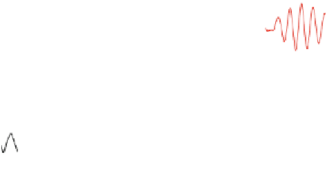
Fig. 12
Comparison of observed variations in polar motion (
black line
) and its corresponding
atmospheric excitation (
red line
) obtained from convolution of the equatorial AAM function for the
time span 1980-2010