Geoscience Reference
In-Depth Information
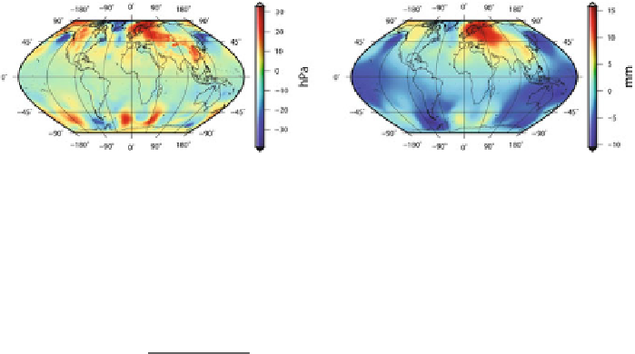
(a)
(b)
Fig. 12 a
Pressure variation (actual-mean) in hPa at 1 January 2008, 00 UTC
b
Resulting geoid
height variation following the TL approach in millimeter
state of the atmosphere, has to be subtracted to obtain the mass variation:
Δ
cos
m
d
S
Earth
(
a
2
λ
C
nm
=
p
s
−
p
s
)
P
nm
(
θ)
.
cos
(33)
Δ
S
nm
sin
m
λ
(
2
n
+
1
)
Mg
0
As an example the first epoch (00 UTC) of 1 January 2008 is selected. Figure
12
a
on the left depicts the pressure variation at the surface and on the right (Fig.
12
b) the
corresponding change in geoid height following the thin layer approach is shown.
3.3.2 3D Atmosphere
As mentioned in the introduction, also the change of the center of mass of the
atmospheric column has an impact on the orbiting satellite, not only the mass change
itself. This variation of the center of mass is not addressed in the thin layer approxi-
mation but has to be taken into account for satellite gravity missions such as GRACE
(Flechtner
2007
; Swenson and Wahr
2002
; Velicogna et al.
2001
). This deficiency
can be overcome by considering the whole vertical structure of the atmosphere by
performing a
vertical integration
(VI) of the atmospheric masses. To do so, Numer-
ical Weather Models which describe the vertical structure by introducing various
numbers of pressure or model levels are needed.
In order to formulate the vertical integration we start from the basic Eqs. (
23
)
and (
27
), introducing the volume element used in Eq. (
32
); for details see (Flechtner
2007
; Zenner et al.
2010
,
2011
).
C
nm
S
nm
cos
m
sin
∞
d
r
P
nm
(
1
λ
r
n
+
2
=−
ρ
cos
θ)
θ
d
θ
d
λ,
Ma
n
sin
m
λ
(
2
n
+
1
)
r
Earth
(34)
Adopting the hydrostatic equation, where
g
r
is the gravity acceleration at each
level, we get: