Path Delays in the Neutral Atmosphere - Atmospheric Effects in Space Geodesy - page 124

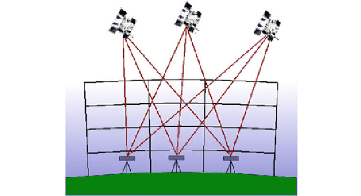
Fig. 16 Example of a GNSS tomography scenario. Note that for better visibility the relative size
of the troposphere have been enlarged; in reality the troposphere ( = top of highest voxel) is about
10 km heigh, the inter-station distances a few km, while the satellites are are at about 20000 km
altitude

in order to reconstruct the 3D structure of the wet (or total) refractivity. This requires
that the slant wet delays are measured by several stations in a local (inter-station
distance maximum a few km) network. The only space geodetic technique for which
such dense networks are available is GNSS.
A picture of a GNSS tomography scenario is shown in Fig. 16 . In order to esti-
mate the wet refractivity field from the observed wet delays, the atmosphere above
the GNSS network is parameterized. The most commonly used parameterization
is voxels, although other parameterizations are also possible (Perler et al. 2011 ).
Voxel parameterization means that the atmosphere is divided into a number of boxes
(called voxels, volume pixels) in which the refractivity is assumed constant. Thus
the wet tropospheric delays along the rays of the observed GNSS signals can be
described by a linear combination of the voxel refractivities

n vox

Δ L i = N j D ij . (199)

j = 1

Δ L i is the wet tropospheric delay along the i th ray, n vox is the number of voxels, N j

is the refractivity of the j th voxel, and D ij is the distance traveled by ray i in voxel j .
Since the station and satellite coordinates are normally known, D ij can be calculated.
Having observations of the tropospheric delays along several different rays, a linear
system of equations is obtained

Δ L = DN . (200)