PEGASUS - Large Scale and Big Data: Processing and Management - page 277

20
18
16
14
12
10
8
6
4
2

Conjecture
by Albert et al.

Sampling

Hadi

Albert
et al.

Hadi

Sampling

Hadi

Directed
Undirected

0.3M 203M

Number of nodes

1.4B

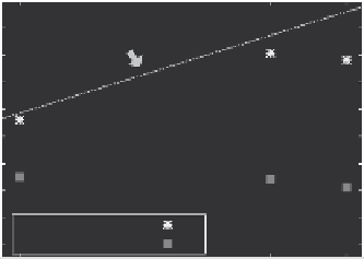
FIGURE 8.17 Average diameter vs. number of vertices in lin-log scale for the three dif-
ferent web graphs, where M and B stand for millions and billions, respectively. (0.3M): web
pages inside nd.edu at 1999, from Albert et al.'s work. (203M): web pages crawled by Altavista
at 1999, from Broder et al.'s work (1.4B): web pages crawled by Yahoo at 2002. Notice the
relatively small diameters for both the directed and the undirected cases.

For the diameter of the undirected graph, we observe the constant/shrinking diam-
eter pattern [32].

8.6.4.2 Shape of Distribution
Figure 8.16 shows that the radii distribution in the web graph is multimodal. In other
relatively smaller networks, we observe a bimodal structure. As shown in the radius
plot of U.S. Patent and LinkedIn network in Figure 8.18, they have a peak at zero, a
dip at a small radius value (9 and 4, respectively) and another peak very close to the
dip.
Observation 2 (Multimodal and Bimodal) The radius distribution of the web
graph has a multimodal structure. Smaller networks have a bimodal structure.
A natural question to ask with respect to the bimodal structure is what are the
common properties of the vertices that belong to the irst peak; similarly, for the
vertices in the irst dip, and the same for the vertices of the second peak. After
investigation, the former are vertices that belong to disconnected components
(DCs); vertices in the dip are usually core vertices in the giant connected com-
ponent (GCC), and the vertices at the second peak are the vast majority of well-
connected vertices in the GCC. Figure 8.19 exactly shows the radii distribution
for the vertices of the GCC (in blue), and the vertices of the few largest remaining
components.
In Figure 8.19, we clearly see that the second peak of the bimodal structure came
from the giant connected component. However, where does the irst peak around
radius 0 come from? We can get the answer from the distribution of connected com-
ponent of the same graph in Figure 8.20. Since the ranges of radius are limited by
the size of connected components, we see the irst peak of radius plot came from the
disconnected components whose size follows a power law.