Information Technology Reference
In-Depth Information
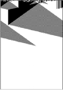
(a)
(b)
Fig.1.
Space-time diagram for the GKL rule. CA cells are depicted horizontally, while
time goes downward. The 0 state is depicted in white; 1 in black. The density of zeros
ρ
0
is 0.476 in (a) and
ρ
0
=0
.
536 in (b).
Table 1.
Performance of the best evolved asynchronous rules calculated over 10
4
bi-
nomially distributed initial configurations. Rule numbers are in hexadecimal.
Update Mode
Rule
Performance
IndependentRandom
00024501006115AF5FFFBFFDE9EFF95F
67
.
2
F ixedRandomSweep
114004060202414150577E771F55FFFF
67
.
7
RandomNewSweep
00520140006013264B7DFCDF4F6DC7DF
65
.
5
from the point of view of the solution strategies that evolved. Since independent
random ordering, i.e. uniform update, is in some sense the more natural, we will
describe it here, although most of what we say also applies to the other two
methods. During most evolutionary runs we observed the presence of periods
in the evolution in which the fitness of the best rules increase in rapid jumps.
These “epochs” were observed in the synchronous case too (see section 3.2) and
correspond to distinct computational innovations, i.e. to major changes in the
strategies that the CA uses for solving the task.
In epoch 1 the evolution only discovers local naive strategies that only work
on “extreme” densities, (i.e. low or high) but most often not on both at the
same time. Fitness is only slightly over 0.5. In the following epoch, epoch 2, rules
specialize on low or high densities as well and use unsophisticated strategies, but
now they give correct results on both low and high densities. This can be seen,
for instance, in figure 2.
In epoch3, withfitness values between 0.80 and 0.90, one sees te emer-
gence of block-expanding strategies, as in the synchronous case, but more noisy.
Moreover, narrow vertical strips appear (see figure 3).