Database Reference
In-Depth Information
Our first step is to define “locality-sensitive functions” generally. We then see how the
idea can be applied in several applications. Finally, we discuss how to apply the theory to
arbitrary data with either a cosine distance or a Euclidean distance measure.
3.6.1
Locality-Sensitive Functions
For the purposes of this section, we shall consider functions that take two items and render
a decision about whether these items should be a candidate pair. In many cases, the func-
tion
f
will “hash” items, and the decision will be based on whether or not the result is equal.
Because it is convenient to use the notation
f
(
x
) =
f
(
y
) to mean that
f
(
x, y
) is “yes; make
x
and
y
a candidate pair,” we shall use
f
(
x
) =
f
(
y
) as a shorthand with this meaning. We also
use
f
(
x
) ≠
f
(
y
) to mean “do not make
x
and
y
a candidate pair unless some other function
concludes we should do so.”
A collection of functions of this form will be called a
family
of functions. For example,
the family of minhash functions, each based on one of the possible permutations of rows of
a characteristic matrix, form a family.
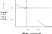
Let
d
1
<
d
2
be two distances according to some distance measure
d
. A family
F
of func-
tions is said to be (
d
1
, d
2
, p
1
, p
2
)
-sensitive
if for every
f
in
F
:
(1) If
d
(
x, y
) ≤
d
1
, then the probability that
f
(
x
) =
f
(
y
) is at least
p
1
.
(2) If
d
(
x, y
) ≥
d
2
, then the probability that
f
(
x
) =
f
(
y
) is at most
p
2
.
d
2
, p
1
, p
2
)-sensitive family will declare two items to be a candidate pair. Notice that we say
nothing about what happens when the distance between the items is strictly between
d
1
and
d
2
, but we can make
d
1
and
d
2
as close as we wish. The penalty is that typically
p
1
and
p
2
are then close as well. As we shall see, it is possible to drive
p
1
and
p
2
apart while keeping
d
1
and
d
2
fixed.
Figure 3.9
Behavior of a (
d
1
,
d
2
,
p
1
,
p
2
)-sensitive function