Information Technology Reference
In-Depth Information
Ta b l e 7 . 7
A statistical hypothesis test for the existence of a linear relationship between
Y
and any of the
X
i
in the regression model of Eq. 7.17
H
0
: β
1
=
β
2
=
β
3
=
...
=
β
k
=
0
H
1
: not all
β
i
(
i
=
1
,...,
k
) are zero.
In conclusion, if the null hypothesis
H
0
is true, no linear relationship exists be-
tween
Y
and any of the independent variables proposed in the regression equation.
On the other hand, if we reject the null hypothesis, there is statistical evidence to
conclude that a regression relationship exists between
Y
and at least one of the in-
dependent variables
X
i
,
i
k
(see 7.7). The
F
test provides what is also called
the
analysis of variance
, based on the localization of the
F
-ratio with respect to the
F
-distribution (with respect to a significance level).
=
1
,...,
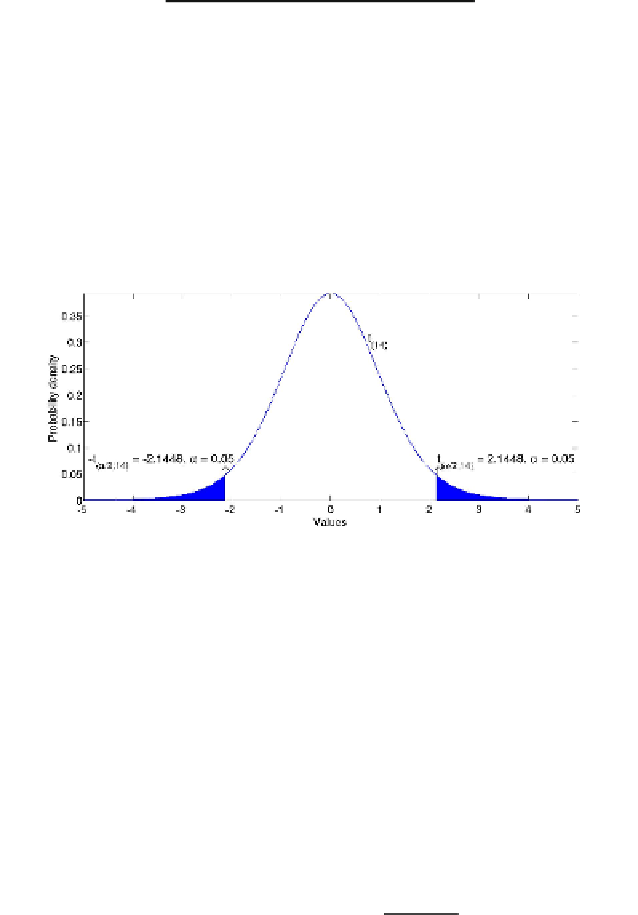
Fig. 7.9
The plot of a
t
-distribution with 14 degrees of freedom
Another probability distribution which is useful in the context of multiple re-
gression is the
Student's t-distribution
(or simply the
t
-distribution), a continuous
probability distribution that is the standard method for evaluating the confidence in-
tervals for a mean when variance is unknown (assuming that population is normally
distributed). Such a kind of distribution is used for calculating the
confidence in-
tervals
for the least squares estimations of the regression coefficients calculated in
(7.18). In statistics, a confidence interval provides the evaluation of the range, of an
estimated parameter, where it is likely to find the correct value of the parameter. This
evaluation is relative to a significance value
α
which gives the probability of being
wrong in the confidence estimation. The
(
1
−
α
)
% confidence interval for each
β
i
,
i
=
0
,...,
k
in Eq. (7.17) is given by:
t
[
α
/
2;
n
−
(
k
+
1
)]
e
ii
·
β
i
=
c
i
±
MSE
,
(7.24)
where
t
[
α
/
2;
n
−
(
k
+
1
)]
is the critical value of a
t
-distribution with
n
−
(
k
+
1
)
degrees of
M
T
)
−
1
freedom for
α
/
2, and
e
ii
is the element in position
(
i
,
i
)
of the matrix
(
×
M
used in Eq. (7.19), which is the sum of the squares of
X
i
(the term
√
e
ii
·
MSE
is the