Mechanisms of Gene Regulation: Boolean Network Models of the Lactose Operon in Escherichia coli - Mathematical Concepts and Methods in Modern Biology - page 25

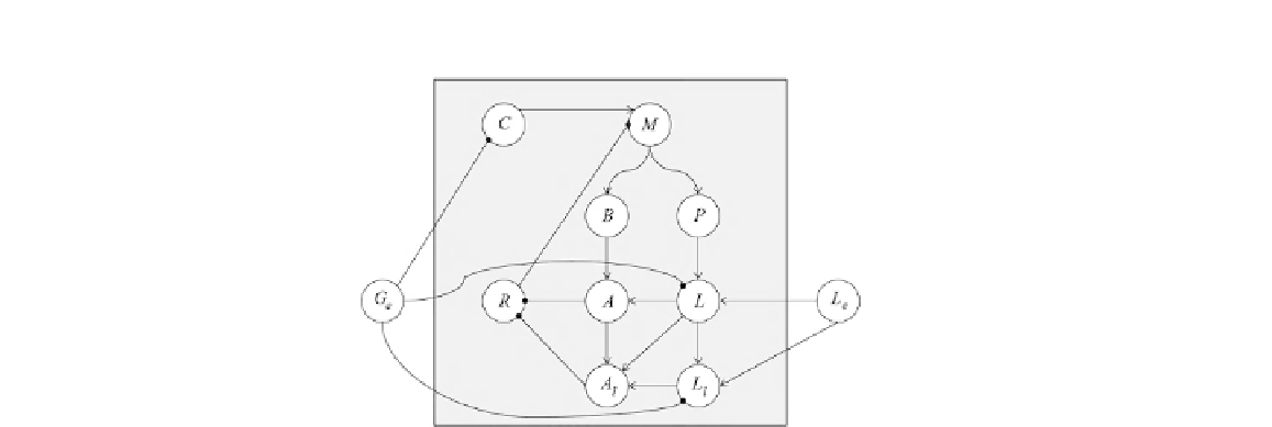
FIGURE 1.11
The wiring diagram for the Boolean model defined by Eqs. ( 1.8 ). The nodes inside the
square region represent model variables, while the outside nodes correspond to model
parameters. Arrows indicate positive interactions, circles indicate negative interactions.
(Figure adapted from Stigler and Veliz-Cuba [ 22 ]).

leading to a state space for the Boolean network model of size 2 9 = 512 for each
of the four combinations of the parameter values. It would be nearly impossible to
compute the individual trajectories of each of these points by hand and determine
the fixed points this way but we may think that a computer would be able to easily
do that. However, for networks with large numbers of nodes, such a “brute force”
approach based on considering all possible trajectories becomes impossible even for
the fastest computers. As an example, a Boolean model of T cell receptor signaling
developed in [ 23 ] contains 94 nodes. This means that the state space contains 2 94
states (approximately equal to 2 10 28 , a number that is about 3,000,000 times larger

than the estimated number of stars in the observable universe [ 24 ]). This means that
years of computing time would be needed even on the fastest computers. Clearly, this
is not practical, implying that DVD and other similar software applications must use
a different, computationally efficient, way to determine the fixed points of a Boolean
network. This justifies the following question: Given a Boolean network model, how
can we determine its fixed points without having to compute the entire state space
transition diagram?

∗

1.4 DETERMINING THE FIXED POINTS OF BOOLEAN
NETWORKS
The dynamical behavior of a Boolean network model with nodes x 1 ,

x 2 ,..., x n is

described by the transition functions f x 1 , f x 2 ,..., f x n , namely