Spatial Modelling and Scaling Issues - Environmental Modelling: Finding Simplicity in Complexity - page 70

observed values. The most well-known example is the
measurement of the length of Britain's coastline, in
which the values change greatly from one measurement
to another when different spatial resolution maps are
used (Mandelbrot, 1982). If the whole of Britain were
reduced to one pixel, the length measurement of the
coastline would be no more than the sum of four pixel
sides. It would be ignored if the pixel size were as large as
whole Europe. In contrast, it would be huge if a measure-
ment scale were less than amillimetre. Obviously, all these
values are not able to represent the reality independently
of scale. In many cases of the natural world, a single value
of a parameter is not meaningful when the measurement
scale is too small or too large. Mandelbrot (1982) intro-
duced the concept of fractals in part to characterize the
way scale changes what is observed. In the next section,
we will discuss an implication for the scaling of model
parameters.
It has been recognized that measured data are an
explicit representation, abstraction or model of some
properties varying in N-dimensional Euclidean space
instead of reality itself (Gatrell, 1991; Burrough and
McDonnell, 1998; Atkinson and Tate, 1999). All the
measured data are a function of the underlying reality
and sampling framework and can generally be described
as the following equation (Atkinson, 1999):

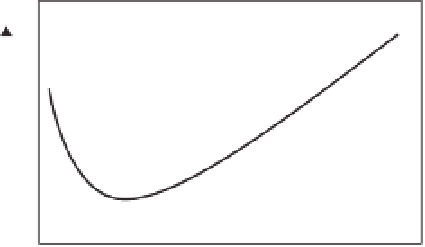
Non-reality

Process
scale

Reality

Small scale Large scale

Figure 5.3 Changes of parameter values with measurement
scales.

the removal of data points to produce a compatible
coarser resolution fromdifferent sources, commonly used
techniques include the averaging method, the thinning
method and dominant values. These methods are simple
and easy to operate but do not deal with the intrinsic
scaling problem. In other cases, we need to find ways
of reproducing the finer details at both coarse and finer
resolutions using a process of interpolation, such as fractal
and geostatistics methods (e.g. kriging), which are more
intricate but robust. With the available of data sources at
multiple scales, particularly remotely sensed data, spatial
environmental modelling tends to use high temporal and
spatial resolution data. In some cases, fine resolution data
with unification and continuity can be produced using
data fusion and calibration methods.
For a grid-based dataset, the averaging method makes
use of the average value over an N by N pixel window
to form a dataset of coarse resolution, which smoothes
the variance of the dataset and increases spatial autocor-
relation. Currently, this is a commonly used technique
for degrading fine-scale remotely sensed data and digital
elevation models (DEMs) (e.g. Helmlinger et al ., 1993;
De Cola, 1997; Hay et al ., 1997). This approach may
reveal the basic relationships involved but simple averag-
ing is unrealistic and may have an effect on the outcome
because there might be nonlinear correlations among
different grids. The thinning method is used to construct
a dataset by subsampling data at fixed intervals, taking
every N th pixel to create a series of coarser data. The
frequency distribution of the sampled data is generally
similar to the original. This method can maximally retain
the variance of the dataset but the information between
every N th pixel is lost.
The dominant method is used to create a coarse res-
olution dataset on the basis of the dominant values in
an N by N window. The variance will be reduced in the

Z ( x ) = f ( Y ( x ), d ) (5.1)

where Z ( x ) is the observed variable, Y ( x ) is the underlying
property and d presents the measurement scale (sampling
framework).
The reality of a variable is associated with its corre-
sponding processes. If a variable is measured at its process
scale, its value can approximate the reality. Otherwise, the
larger (or smaller) the measurement scales compared to
the process scale, themoremeaningless the variable values
(Figure 5.3). For example, when using remotely sensed
data to classify land cover, the resultant land-cover map
will be most accurate when using approximately field-
sized pixels. If pixels either much smaller or much larger
than a typical field are used, classification accuracy will
consequently decrease (Woodcock et al ., 1988a, 1988b;
Curran and Atkinson, 1999). Because of the complexity
of natural environments, there are no universal guidelines
for deciding the process scales.

5.4.2 Methodsof scalingparameters

Techniques are often required to relate information at
one spatial scale to another. In some cases that involve