Non-Linear Dynamics, Self-Organization and Cellular Automata Models - Environmental Modelling: Finding Simplicity in Complexity - page 56

4.4.2 TheRillGrow2model

RillGrow 2, like RillGrow 1, operates upon an area of bare
soil, which is specified as a grid of microtopographic ele-
vations (a DEM). Typically, cell size is a few millimetres,
with elevation data either derived from real soil surfaces
(Figure 4.3) by using a laser scanner (Huang and Bradford,
1992) or by means of photogrammetry (Lascelles et al .,
2002); or generated using some random function (cf.
Favis-Mortlock, 1998b). Computational constraints
mean that, for practical purposes, the microtopographic
grid can be no larger than plot-sized. A gradient is usually
imposed on this grid. The model operates has a variable
timestep, which is typically of the order of 0.05 s. At each
timestep, multiple raindrops are dropped at random
locations on the grid, with the number of drops depend-
ing on rainfall intensity. Runon from upslope may also be
added at an edge of the grid. Often, the soil is assumed to
be fully saturated so that no infiltration occurs; however
a fraction of all surface water may be removed each
timestep as a crude representation of infiltration losses.
Splash redistribution is simulated in RillGrow 2. Since
this is a relatively slow process it is not normally calculated
every timestep. The relationship by Planchon et al . (2000)
is used: this is essentially a diffusion equation based on
the Laplacian, with a 'splash-efficiency' term, which is a
function of rainfall intensity and water depth. Currently,
the splash redistribution and overland flow components
of RillGrow 2 are only loosely coupled: while sediment
which is redistributed by splash can be moved in or out of
the store of flow-transported sediment, this is not done
in an explicitly spatial manner.

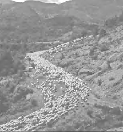
Figure 4.4 'Sheepflow': a visual analogy of RillGrow 2's
discretized representation of overland flow. Which should a
modeller best focus on: the movement of an individual sheep or
the 'flow' of the flock of sheep? Photograph Martin Price,

1999 [e-mail]), used by permission.

Movement of overland flow between 'wet' cells occurs
in discrete steps between cells of this grid. Conceptually,
overland flow in RillGrow 2 is therefore a kind of
discretized fluid rather like the 'sheepflow' illustrated
in Figure 4.4.
For the duration of the simulation, each 'wet' cell is
processed in a random sequence which varies at each
timestep. The simple logic outlined in Figure 4.5 is used
for the processing.
Outflow may occur from a 'wet' cell to any of the eight
adjacent cells. If outflow is possible, the direction with
the steepest energy gradient (i.e. maximum difference in
water-surface elevation) is chosen. The potential velocity
of this outflow is calculated as a function of water depth
and hydraulic radius. However outflow only occurs if
sufficient time has elapsed for the water to have crossed
this cell. Thus outflow only occurs for a subset of 'wet'
cells at each timestep.
When outflow does occur, the transport capacity of
the flow is calculated using the previously calculated flow
velocity with this S-curve relationship (equation 5 in
Nearing et al ., 1997):

Figure 4.3 Soil surface microtopography: the scale at which
RillGrow 2's rules operate. The finger indicates where flow
(from right to left) is just beginning to incise a microrill in a
field experiment (see Lascelles et al ., 2000). Photograph

Martin Barfoot, 1997 [e-mail]), used by
permission.

e γ + δ · log e ( ω ) α + β ·

log e ( q s ) = (4.1)

e γ + δ · log e ( ω ) 1 +