Environmental Engineering Reference
In-Depth Information
100,000,000
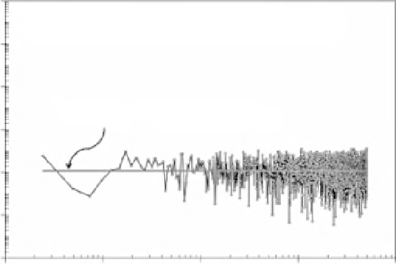
Periodogram of White noise
1,000,000
10,000
S
m
= 1.12
f
m
−
0.003
S
m
100
1
0.01
0.0001
0.0001
0.001
0.01
f
m
0.1
1
(a)
100,000,000
Periodogram of Brownian Motion
1,000,000
10,000
S
m
100
S
m
= 0.0167
f
m
−
1.993
1
0.01
0.0001
0.0001
0.001
0.01
f
m
0.1
1
(b)
Figure 3.7
Power-spectral analysis applied to (a) an equally spaced Gaussian white noise with mean
x
=
0
.
0 and standard deviation
σ
x
=
4096 values; shorter examples
are shown in Figure 3.4. The resultant periodograms for each case are shown, where the power-spectral density function
S
m
from
Equation 3.12 is given as a function of frequency
f
m
=
1
.
0, and (b) a Brownian motion, the running sum of the white noise. Both time series have
N
=
δ
=
...
/
δ
=
m
/(
N
),
m
1, 2, 3,
,
N
2, and
1 (no units). Also shown are the best
β
β
fits of Equation 3.13, with
the negative of the power-law exponent;
is a measure of the strength of the long-range persistence, if it
exists.
values are correlated relative to a Gaussian white noise
(
fractional Brownian motions
(non-stationary time series).
This relationship is true for any symmetrical frequency-
size distribution (e.g. the Gaussian) and long-range
persistent time series, so that the running sum will result
in a time series with
β
shifted by
+
2
.
0. In Figure 3.8,
we sum the fractional Gaussian noises in the left column,
with
β
=−
1
.
0,
−
0
.
5,
+
0
.
5,
+
1
.
0, to give the fractional
Brownian walks (shown in the right column of Figure 3.8)
β
=
0). For these persistent time series, values larger
than the mean tend to be followed by a value larger than
the mean.
Just as previously we summed a Gaussian white noise
with
β
=
β
=
.
0
(Equation 3.4, Figure 3.4), one can also sum
fractional
Gaussian noises
(weakly stationary time series) to give
0 to give a Brownian motion with
2


Search WWH ::

Custom Search