Assessing Model Adequacy - Environmental Modelling: Finding Simplicity in Complexity - page 431

2 for al l x a , and th e correlation between any
two residuals f t ( x a )and f t ( x a ) is taken to be of the

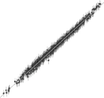
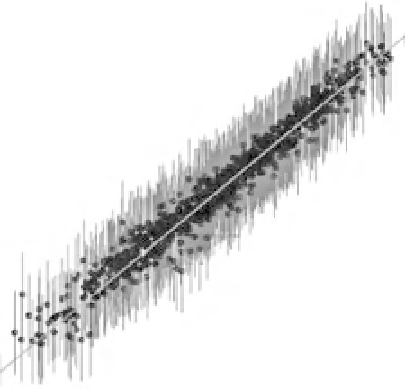
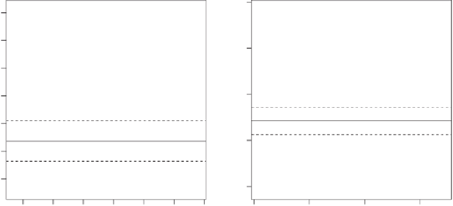
with the model outputs. Figure 26.6 illustrates results
(using just 1000 randomly selected points from the
100 000) for the emulators at 460 hours (left panel)
and 820 hours (right panel). Each panel shows the
emulated logarithm of discharge with three emula-
tor standard deviation limits versus the corresponding
100 000 model values, the 1:1 line and the field obser-
vation value with three measurement error standard
deviation limits. Clearly the emulator at 460 hours is
more accurate than that for 820 hours. It can also be
seen that both emulators are satisfactory in that a large
number of prediction intervals (shown as error bars)
do indeed cover the correct model discharge values
represented by the 1:1 line. Notice that for both hours
there are model runs that match the field data within
the measurement error limits, suggesting good fits.
However, while we find that this is also true for the
other 11 hours, we cannot be sure there is a common
set of inputs at which the model runs for all 13 hours
fit well, or indeed for all 839 hours, a point we address
in the next section.

(1 − δ ) σ

2 for any two inputs x
and x with active input components x a and x a , where
θ k , which is either chosen or estimated, controls the
contribution to the overall correlation between the
corresponding two outputs in the direction of the k th
active input component x a .Wechoseeach θ k = 0 . 33,
one-third of the length an input interval, a choice
based on previous experience of fitting quadratics to
computer-model output
7. We check emulator accuracy by evaluating it at the
inputs of an additional set of evaluation or diagnostic
model runs to see whether the emulator evalua-
tions at these inputs are 'close' to the corresponding
model outputs, where for each evaluation, closeness
is assessed with respect to the standard deviation
of the emulator at the evaluation input. We would
normally choose a small number of diagnostic runs
(about 100) with inputs in a Latin hypercube, modified
to accommodate the sum-to-one restriction. However,
for demonstration purposes we use the 13 emulators to
obtain emulator expectation and variances at the same
100 000 points used in Section 26.3 to obtain a more
detailed assessment of the emulators in comparison

form exp − k x ( k )

− x a ( k )
θ k

a

26.4.1 Implausibility

The definition of implausibility for slow computermodels
is similar to that for fast models given in Equation 26.7
(see, for example, Craig et al ., 2001). We define the

− 4.4 − 4.2 − 4.0 − 3.8

Discharge

− 3.6 − 3.4 − 3.2 − 4.0 − 3.5 − 3.0 − 2.5

Discharge

Figure 26.6 Emulated logarithm of discharge (dots) with three emulator standard deviation limits (line segments) versus the
corresponding randomly chosen 1000 runoff model values from 100 000 runs; the 1:1 line; and field observation value (black line)
with three measurement error standard deviation limits (black dotted lines) for the emulators at 460 hours (left panel) and 820 hours
(right panel).