Environmental Engineering Reference
In-Depth Information
0.40
Erica scoparia
0.40
Erica scoparia
0.30
0.30
0.20
0.20
0.10
0.10
0.00
0.00
0.20
Rubus ulmifolius
0.20
Rubus ulmifolius
0.15
0.15
0.10
0.05
0.10
0.00
0.05
0.00
0.06
Ulex jussiaeu
0.06
Ulex jussiaeu
0.04
0.04
0.02
0.02
0
0
10
20
Months after fire
30
40
0
0
10
20
Months after fire
30
40
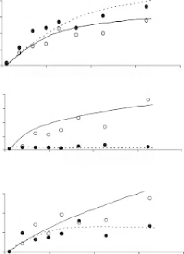
Figure 14.4
Results of system dynamic model simulation of
cover changes of three competing species according to grazing
treatment. Data are the same as those reported in Figure 14.2.
Solid lines and open symbols represent protected plots. Dashed
lines and closed symbols represent grazed plots.
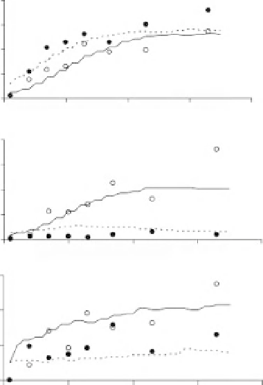
Figure 14.5
Results of individual-based model simulation of
cover changes of three competing species according to grazing
treatment. Data are the same reported in Figure 14.2. Solid lines
and open symbols represent protected plots. Dashed lines and
closed symbols represent grazed plots.
continuous way. For this reason, it was manageable using
differential equations. In the IBM, the focus of the model
is shifted from species cover to properties of individual
plant. In this type of model representation, vegetation
cover is then the result of the covers of the assemblage of
competing individual plants of the different species.
We can create a class of plant individuals with two rules
equivalent in their algorithmic structure and evaluated at
each timestep. In the first rule, which deals with plant
mortality, each individual 'draws' a random number, and
depending on whether its value is less than the plant's
assigned probability of dying, it perishes or not. The same
algorithm is used in the second rule to compute seed
dispersal. Soil carrying capacity and fire/grazing effects
act as modifiers to the abovementioned probabilities.
The application of this modelling approach can pro-
duce a simulation of population dynamics showing
both individual life-span patterns and aggregated species
behaviours. The emergent trends of species dominance
reflect the same dynamics observed for the ordinary
differential equations model of the previous example
(Figure 14.5).
0.6
No Grazing
Ulex jussiaeu
0.4
Erica scoparia
0.2
Rubus ulmifolius
0
.6
Grazing
Erica scoparia
0.4
Ulex jussiaeu
0.2
Rubus ulmifolius
0
0
5
10
15
Time (years)
20
25
30
Figure 14.6
Long-term modelled successional changes
according to grazing disturbance.


Search WWH ::

Custom Search